{x}
blog image

Maximum Genetic Difference Query

There is a rooted tree consisting of n nodes numbered 0 to n - 1. Each node's number denotes its unique genetic value (i.e. the genetic value of node x is x). The genetic difference between two genetic values is defined as the bitwise-XOR of their values. You are given the integer array parents, where parents[i] is the parent for node i. If node x is the root of the tree, then parents[x] == -1.

You are also given the array queries where queries[i] = [nodei, vali]. For each query i, find the maximum genetic difference between vali and pi, where pi is the genetic value of any node that is on the path between nodei and the root (including nodei and the root). More formally, you want to maximize vali XOR pi.

Return an array ans where ans[i] is the answer to the ith query.


Example 1:

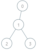
Input: parents = [-1,0,1,1], queries = [[0,2],[3,2],[2,5]]
Output: [2,3,7]
Explanation: The queries are processed as follows:
- [0,2]: The node with the maximum genetic difference is 0, with a difference of 2 XOR 0 = 2.
- [3,2]: The node with the maximum genetic difference is 1, with a difference of 2 XOR 1 = 3.
- [2,5]: The node with the maximum genetic difference is 2, with a difference of 5 XOR 2 = 7.

Example 2:

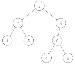
Input: parents = [3,7,-1,2,0,7,0,2], queries = [[4,6],[1,15],[0,5]]
Output: [6,14,7]
Explanation: The queries are processed as follows:
- [4,6]: The node with the maximum genetic difference is 0, with a difference of 6 XOR 0 = 6.
- [1,15]: The node with the maximum genetic difference is 1, with a difference of 15 XOR 1 = 14.
- [0,5]: The node with the maximum genetic difference is 2, with a difference of 5 XOR 2 = 7.


Constraints:

  • 2 <= parents.length <= 105
  • 0 <= parents[i] <= parents.length - 1 for every node i that is not the root.
  • parents[root] == -1
  • 1 <= queries.length <= 3 * 104
  • 0 <= nodei <= parents.length - 1
  • 0 <= vali <= 2 * 105

Solution Explanation for Maximum Genetic Difference Query

This problem involves finding the maximum genetic difference between a given value and all nodes along a path from a specified node to the root of a tree. The genetic difference is calculated using bitwise XOR. The solution efficiently handles this using Depth-First Search (DFS) and a Trie data structure.

Approach:

  1. Build the Tree: Construct the tree structure from the parents array. Each element in parents indicates the parent of the corresponding node. A node with parents[i] == -1 is the root.

  2. DFS for Path Traversal: Perform a Depth-First Search (DFS) to traverse the tree. For each query [node, val], DFS is initiated from the given node. During the traversal, we collect all genetic values (node numbers) encountered along the path from the given node to the root.

  3. Trie for Efficient XOR Maximization: A Trie (prefix tree) is used to efficiently find the maximum XOR value with val. Each Trie node represents a bit (0 or 1). When inserting a genetic value into the Trie, we traverse down the tree according to the bits of the value. To find the maximum XOR with val, we traverse the Trie, choosing the bit that maximizes the XOR at each level.

  4. Query Processing: For each query [node, val], we perform the DFS to get the path to the root. Then, we iterate through the path's genetic values, inserting them into the Trie. Finally, we query the Trie to find the maximum XOR with val. This process is repeated for each query.

Time Complexity Analysis:

  • Tree Building: O(N), where N is the number of nodes in the tree.
  • DFS: O(N) in the worst case (a skewed tree).
  • Trie Insertion/Query: O(log M) per node, where M is the maximum genetic value (node number). In total, this becomes O(N log M) for all nodes.
  • Query Processing: O(Q * (N + log M)), where Q is the number of queries. The N comes from the DFS and log M comes from the Trie query.

Therefore, the overall time complexity is dominated by the query processing step, resulting in O(Q * (N + log M)). The space complexity is O(N + Q + M log M), due to the tree, query results, and Trie. The log M factor in the Trie space complexity is because the height of the trie is proportional to the number of bits in the maximum value M.

Code (Python):

class TrieNode:
    def __init__(self):
        self.children = [None, None]  # 0 and 1 children
 
class Trie:
    def __init__(self):
        self.root = TrieNode()
 
    def insert(self, val):
        node = self.root
        for i in range(17, -1, -1):  # Assuming max val < 2^18
            bit = (val >> i) & 1
            if node.children[bit] is None:
                node.children[bit] = TrieNode()
            node = node.children[bit]
 
    def query(self, val):
        max_xor = 0
        node = self.root
        for i in range(17, -1, -1):
            bit = (val >> i) & 1
            if node.children[1 - bit] is not None:
                max_xor |= (1 << i)
                node = node.children[1 - bit]
            else:
                node = node.children[bit]
        return max_xor
 
 
def maxGeneticDifference(parents, queries):
    n = len(parents)
    adj = [[] for _ in range(n)]
    for i, p in enumerate(parents):
        if p != -1:
            adj[p].append(i)
 
    ans = []
    trie = Trie()
 
    def dfs(u, path):
        path.append(u)
        for node in path:
            trie.insert(node)
        for v in adj[u]:
            dfs(v, path.copy())  # important to use copy for independent path
 
    for node, val in queries:
        path = []
        dfs(node, path)
        ans.append(trie.query(val))
        trie = Trie() #Reset Trie for next Query
 
 
    return ans
 

Other Languages: The core logic remains the same for other languages like Java or C++. The primary differences would be in the implementation details of the Trie and tree structures, but the algorithmic approach would stay consistent. You would need to adapt the code to handle memory management and potentially use different data structures for efficiency in those languages.