Given the root
of a binary tree, return the leftmost value in the last row of the tree.
Example 1:
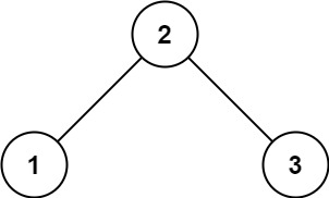
Input: root = [2,1,3] Output: 1
Example 2:
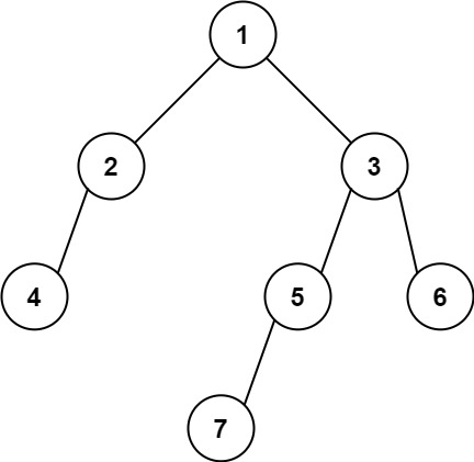
Input: root = [1,2,3,4,null,5,6,null,null,7] Output: 7
Constraints:
[1, 104]
.-231 <= Node.val <= 231 - 1
This problem asks to find the leftmost value in the last row of a binary tree. We can solve this using either Breadth-First Search (BFS) or Depth-First Search (DFS).
This approach is generally more intuitive and efficient for level-order traversal. We use a queue to store nodes level by level. In each level, the first node encountered will be the leftmost node at that level. The last level's leftmost node is our answer.
Algorithm:
Initialization: Create a queue q
and add the root node to it. Initialize a variable ans
to store the leftmost value.
Level-Order Traversal: While the queue is not empty:
ans
with the value of the first node in the queue (this is the leftmost node at the current level).Return: After the loop, ans
holds the leftmost value of the last row.
Time Complexity: O(N), where N is the number of nodes in the tree. Each node is visited and processed exactly once.
Space Complexity: O(W), where W is the maximum width of the tree. In the worst case (a complete binary tree), W can be equal to N, but in practice it's often much smaller. The space complexity is dominated by the queue used in BFS.
This approach uses a recursive Depth-First Search. We keep track of the maximum depth encountered so far and the corresponding leftmost value.
Algorithm:
Initialization: Initialize ans
(the leftmost value) and mx
(the maximum depth) to 0.
Recursive DFS: Implement a recursive function dfs(root, curr)
that takes the current node and its depth curr
as input.
root
is None
, return.dfs
for the left and right subtrees, incrementing the depth.ans
and mx
: If the current depth curr
is greater than mx
, it means we've reached a deeper level. Update mx
to curr
and ans
to root.val
.Return: After the recursive calls finish, ans
will contain the leftmost value at the maximum depth.
Time Complexity: O(N), as each node is visited exactly once.
Space Complexity: O(H), where H is the height of the tree. This is due to the recursive call stack. In the worst case (a skewed tree), H can be equal to N.
The code examples for both approaches are provided in the original response. I'll highlight key aspects:
BFS (Python):
from collections import deque
class Solution:
def findBottomLeftValue(self, root: Optional[TreeNode]) -> int:
q = deque([root])
ans = 0
while q:
ans = q[0].val # Leftmost at current level
for _ in range(len(q)):
node = q.popleft()
if node.left:
q.append(node.left)
if node.right:
q.append(node.right)
return ans
DFS (Python):
class Solution:
def findBottomLeftValue(self, root: Optional[TreeNode]) -> int:
ans = mx = 0 # ans: leftmost value, mx: max depth
def dfs(root, curr):
nonlocal ans, mx
if not root: return
dfs(root.left, curr + 1)
dfs(root.right, curr + 1)
if curr > mx: # Found a deeper level
mx = curr
ans = root.val
dfs(root, 1)
return ans
The code in other languages (Java, C++, Go, TypeScript, Rust) follow similar logic and structure to these Python examples. Choose the approach (BFS or DFS) that best suits your understanding and coding style. Generally, BFS is preferred for level-order traversals due to its better space complexity in many practical scenarios.