You are given two integers m
and n
representing a 0-indexed m x n
grid. You are also given two 2D integer arrays guards
and walls
where guards[i] = [rowi, coli]
and walls[j] = [rowj, colj]
represent the positions of the ith
guard and jth
wall respectively.
A guard can see every cell in the four cardinal directions (north, east, south, or west) starting from their position unless obstructed by a wall or another guard. A cell is guarded if there is at least one guard that can see it.
Return the number of unoccupied cells that are not guarded.
Example 1:
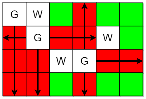
Input: m = 4, n = 6, guards = [[0,0],[1,1],[2,3]], walls = [[0,1],[2,2],[1,4]] Output: 7 Explanation: The guarded and unguarded cells are shown in red and green respectively in the above diagram. There are a total of 7 unguarded cells, so we return 7.
Example 2:
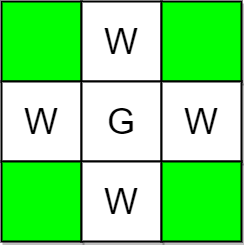
Input: m = 3, n = 3, guards = [[1,1]], walls = [[0,1],[1,0],[2,1],[1,2]] Output: 4 Explanation: The unguarded cells are shown in green in the above diagram. There are a total of 4 unguarded cells, so we return 4.
Constraints:
1 <= m, n <= 105
2 <= m * n <= 105
1 <= guards.length, walls.length <= 5 * 104
2 <= guards.length + walls.length <= m * n
guards[i].length == walls[j].length == 2
0 <= rowi, rowj < m
0 <= coli, colj < n
guards
and walls
are unique.This problem involves finding the number of unguarded cells in a grid given the positions of guards and walls. Guards can see in four directions (north, east, south, west) until obstructed by a wall or another guard.
This approach uses a simulation to determine which cells are guarded. We represent the grid using a 2D array.
Initialization: Create a grid g
of size m x n
filled with zeros (0 represents unguarded, 1 represents guarded, 2 represents wall/guard). Mark the positions of guards and walls with 2 in g
.
Guard Simulation: Iterate through each guard's position. For each guard, simulate its line of sight in each of the four directions (up, down, left, right). In each direction:
Unguarded Cell Count: Finally, iterate through the grid g
. Count the number of cells with a value of 0; these are the unguarded cells. Return this count.
g
to represent the grid, which has a size of m x n
.This approach uses Depth-First Search (DFS) to simulate the line of sight of each guard.
Initialization: Similar to Approach 1, create a grid and mark guard and wall positions as 2.
DFS Function: A recursive DFS function takes the current cell coordinates, the direction vector (dx, dy), and recursively explores the line of sight in that direction, marking guarded cells as 1. It stops when it encounters a wall or boundary.
Guard Traversal: Iterate through guards and, for each guard, call the DFS function for all four directions.
Unguarded Cell Count: Calculate the number of unguarded cells by subtracting the number of guards, walls, and guarded cells from the total number of cells (m*n).
mtx
dominates the space complexity. The recursive call stack of the DFS is at most O(min(m,n)) in depth.Python:
def countUnguarded(m, n, guards, walls):
grid = [[0] * n for _ in range(m)]
for r, c in guards:
grid[r][c] = 2
for r, c in walls:
grid[r][c] = 2
for r, c in guards:
for dr, dc in [(0, 1), (0, -1), (1, 0), (-1, 0)]:
nr, nc = r + dr, c + dc
while 0 <= nr < m and 0 <= nc < n and grid[nr][nc] < 2:
grid[nr][nc] = 1
nr += dr
nc += dc
return sum(sum(cell == 0 for cell in row) for row in grid)
JavaScript:
function countUnguarded(m, n, guards, walls) {
const grid = Array.from({ length: m }, () => Array(n).fill(0));
for (const [r, c] of guards) grid[r][c] = 2;
for (const [r, c] of walls) grid[r][c] = 2;
for (const [r, c] of guards) {
for (const [dr, dc] of [[0, 1], [0, -1], [1, 0], [-1, 0]]) {
let nr = r + dr, nc = c + dc;
while (nr >= 0 && nr < m && nc >= 0 && nc < n && grid[nr][nc] < 2) {
grid[nr][nc] = 1;
nr += dr;
nc += dc;
}
}
}
return grid.flat().filter(cell => cell === 0).length;
}
The other languages (Java, C++, Go, TypeScript) would follow a similar structure, adapting the syntax to their respective languages. The core logic remains the same across all implementations. Choose the approach and language that best suits your needs and understanding. Approach 1 (Simulation) is generally easier to understand, while Approach 2 (DFS) might be slightly more efficient in specific cases but adds a layer of recursion.