{x}
blog image

Unique Paths II

You are given an m x n integer array grid. There is a robot initially located at the top-left corner (i.e., grid[0][0]). The robot tries to move to the bottom-right corner (i.e., grid[m - 1][n - 1]). The robot can only move either down or right at any point in time.

An obstacle and space are marked as 1 or 0 respectively in grid. A path that the robot takes cannot include any square that is an obstacle.

Return the number of possible unique paths that the robot can take to reach the bottom-right corner.

The testcases are generated so that the answer will be less than or equal to 2 * 109.


Example 1:

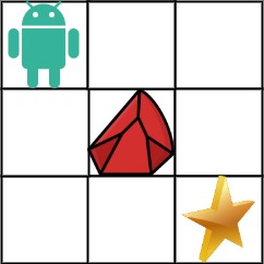
Input: obstacleGrid = [[0,0,0],[0,1,0],[0,0,0]]
Output: 2
Explanation: There is one obstacle in the middle of the 3x3 grid above.
There are two ways to reach the bottom-right corner:
1. Right -> Right -> Down -> Down
2. Down -> Down -> Right -> Right

Example 2:

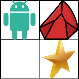
Input: obstacleGrid = [[0,1],[0,0]]
Output: 1


Constraints:

  • m == obstacleGrid.length
  • n == obstacleGrid[i].length
  • 1 <= m, n <= 100
  • obstacleGrid[i][j] is 0 or 1.

Solution Explanation for Unique Paths II

This problem asks to find the number of unique paths a robot can take from the top-left corner to the bottom-right corner of a grid, given that some cells are obstacles (marked as 1) and the robot can only move down or right.

Two approaches are presented: Memoization (recursive with caching) and Dynamic Programming (iterative). Both achieve the same result but differ in implementation and efficiency characteristics.

Approach 1: Memoization Search (Recursive with Caching)

This approach uses recursion to explore all possible paths. The dfs(i, j) function recursively counts the paths from cell (i, j) to the destination.

  • Base Cases:
    • If (i, j) is out of bounds or an obstacle, there are no paths (return 0).
    • If (i, j) is the destination, there's one path (return 1).
  • Recursive Step: Otherwise, the number of paths from (i, j) is the sum of paths from (i+1, j) (moving down) and (i, j+1) (moving right).

Memoization: To avoid redundant calculations, a cache (@cache in Python, f[][] in other languages) stores the results of dfs(i, j). If a result is already cached, it's directly returned, improving efficiency.

Time Complexity: O(m*n), where 'm' and 'n' are the dimensions of the grid. Each cell is visited at most once due to memoization.

Space Complexity: O(m*n) for the cache. The recursive call stack could also consume space in the worst case, but memoization significantly reduces its depth.

Approach 2: Dynamic Programming (Iterative)

This approach builds a DP table f[i][j] where f[i][j] stores the number of paths to reach cell (i, j).

  • Initialization:
    • f[0][0] = 1 if it's not an obstacle; otherwise, it's 0.
    • The first row and column are initialized based on obstacle presence: if there's an obstacle at (i, 0) or (0, j), the values in the respective row/column become 0 after that point; otherwise they remain 1.
  • Iteration: The table is filled iteratively:
    • If obstacleGrid[i][j] == 0, then f[i][j] = f[i-1][j] + f[i][j-1] (paths from above + paths from the left).
    • Otherwise, f[i][j] = 0.
  • Result: f[m-1][n-1] contains the total number of paths to the destination.

Time Complexity: O(m*n). The table is filled in a single pass.

Space Complexity: O(m*n) for the DP table.

Code Examples (Multiple Languages)

The code examples for both approaches are provided in the problem statement. They demonstrate how to implement these approaches in Python, Java, C++, Go, TypeScript, Rust, and Javascript. The dynamic programming solutions are generally slightly more concise. The choice between memoization and dynamic programming often depends on personal preference and coding style; for this specific problem, the performance differences are minimal in practice.