
Rank Transform of a Matrix
Given an m x n matrix, return a new matrix answer where answer[row][col] is the rank of matrix[row][col].
The rank is an integer that represents how large an element is compared to other elements. It is calculated using the following rules:
- The rank is an integer starting from
1. - If two elements
pandqare in the same row or column, then:- If
p < qthenrank(p) < rank(q) - If
p == qthenrank(p) == rank(q) - If
p > qthenrank(p) > rank(q)
- If
- The rank should be as small as possible.
The test cases are generated so that answer is unique under the given rules.
Example 1:
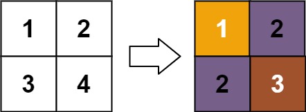
Input: matrix = [[1,2],[3,4]]
Output: [[1,2],[2,3]]
Explanation:
The rank of matrix[0][0] is 1 because it is the smallest integer in its row and column.
The rank of matrix[0][1] is 2 because matrix[0][1] > matrix[0][0] and matrix[0][0] is rank 1.
The rank of matrix[1][0] is 2 because matrix[1][0] > matrix[0][0] and matrix[0][0] is rank 1.
The rank of matrix[1][1] is 3 because matrix[1][1] > matrix[0][1], matrix[1][1] > matrix[1][0], and both matrix[0][1] and matrix[1][0] are rank 2.
Example 2:
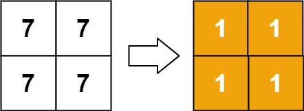
Input: matrix = [[7,7],[7,7]]
Output: [[1,1],[1,1]]
Example 3:
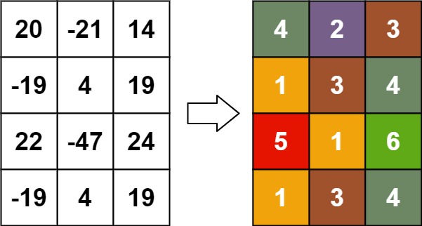
Input: matrix = [[20,-21,14],[-19,4,19],[22,-47,24],[-19,4,19]]
Output: [[4,2,3],[1,3,4],[5,1,6],[1,3,4]]
Constraints:
m == matrix.lengthn == matrix[i].length1 <= m, n <= 500-109 <= matrix[row][col] <= 109
On This Page
Also Explore
DSA Questions
Largest Substring Between Two Equal Characters
DSA Questions
Best Team With No Conflicts
DSA Questions
Graph Connectivity With Threshold
DSA Questions
Design an Expression Tree With Evaluate Function
DSA Questions
Slowest Key
DSA Questions
Arithmetic Subarrays
DSA Questions
Path With Minimum Effort
DSA Questions
Rank Transform of a Matrix
DSA Questions
Percentage of Users Attended a Contest
DSA Questions
Add Two Polynomials Represented as Linked Lists
DSA Questions
Hopper Company Queries I
DSA Questions
Sort Array by Increasing Frequency
DSA Questions
Count Substrings That Differ by One Character
DSA Questions