
Path with Maximum Probability
You are given an undirected weighted graph of n nodes (0-indexed), represented by an edge list where edges[i] = [a, b] is an undirected edge connecting the nodes a and b with a probability of success of traversing that edge succProb[i].
Given two nodes start and end, find the path with the maximum probability of success to go from start to end and return its success probability.
If there is no path from start to end, return 0. Your answer will be accepted if it differs from the correct answer by at most 1e-5.
Example 1:
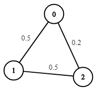
Input: n = 3, edges = [[0,1],[1,2],[0,2]], succProb = [0.5,0.5,0.2], start = 0, end = 2
Output: 0.25000
Explanation: There are two paths from start to end, one having a probability of success = 0.2 and the other has 0.5 * 0.5 = 0.25.
Example 2:
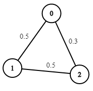
Input: n = 3, edges = [[0,1],[1,2],[0,2]], succProb = [0.5,0.5,0.3], start = 0, end = 2
Output: 0.30000
Example 3:
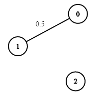
Input: n = 3, edges = [[0,1]], succProb = [0.5], start = 0, end = 2
Output: 0.00000
Explanation: There is no path between 0 and 2.
Constraints:
2 <= n <= 10^40 <= start, end < nstart != end0 <= a, b < na != b0 <= succProb.length == edges.length <= 2*10^40 <= succProb[i] <= 1- There is at most one edge between every two nodes.
On This Page
Also Explore
DSA Questions
Find Root of N-Ary Tree
DSA Questions
Reformat Date
DSA Questions
Range Sum of Sorted Subarray Sums
DSA Questions
Stone Game IV
DSA Questions
Customer Order Frequency
DSA Questions
Number of Good Pairs
DSA Questions
Number of Substrings With Only 1s
DSA Questions
Path with Maximum Probability
DSA Questions
Best Position for a Service Centre
DSA Questions
Move Sub-Tree of N-Ary Tree
DSA Questions
Find Users With Valid E-Mails
DSA Questions
Water Bottles
DSA Questions
Number of Nodes in the Sub-Tree With the Same Label
DSA Questions
Maximum Number of Non-Overlapping Substrings
DSA Questions