{x}
blog image

Best Position for a Service Centre

A delivery company wants to build a new service center in a new city. The company knows the positions of all the customers in this city on a 2D-Map and wants to build the new center in a position such that the sum of the euclidean distances to all customers is minimum.

Given an array positions where positions[i] = [xi, yi] is the position of the ith customer on the map, return the minimum sum of the euclidean distances to all customers.

In other words, you need to choose the position of the service center [xcentre, ycentre] such that the following formula is minimized:

Answers within 10-5 of the actual value will be accepted.


Example 1:

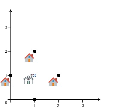
Input: positions = [[0,1],[1,0],[1,2],[2,1]]
Output: 4.00000
Explanation: As shown, you can see that choosing [xcentre, ycentre] = [1, 1] will make the distance to each customer = 1, the sum of all distances is 4 which is the minimum possible we can achieve.

Example 2:

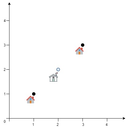
Input: positions = [[1,1],[3,3]]
Output: 2.82843
Explanation: The minimum possible sum of distances = sqrt(2) + sqrt(2) = 2.82843


Constraints:

  • 1 <= positions.length <= 50
  • positions[i].length == 2
  • 0 <= xi, yi <= 100

Solution Explanation: Finding the Best Position for a Service Center

This problem asks to find the optimal location for a service center that minimizes the total Euclidean distance to all customers. A brute-force approach is computationally expensive. Instead, we can use an iterative optimization technique, specifically a gradient descent method, to approximate the optimal solution efficiently.

Approach:

  1. Initialization: Start with an initial guess for the service center's coordinates (x, y). A reasonable starting point is the centroid of all customer positions (average x and y coordinates).

  2. Gradient Calculation: Calculate the gradient of the total distance function at the current (x, y) point. The gradient indicates the direction of the steepest ascent. We want to move in the opposite direction (steepest descent) to minimize the total distance. The gradient components are calculated by summing the partial derivatives of the distance from each customer to the service center with respect to x and y.

  3. Update Coordinates: Update the (x, y) coordinates of the service center by moving a small step in the opposite direction of the gradient. The step size is controlled by a learning rate (alpha).

  4. Iteration and Convergence: Repeat steps 2 and 3 until the gradient becomes sufficiently small (indicating we are near a minimum) or a maximum number of iterations is reached. To ensure convergence, we can gradually reduce the step size (alpha) using a decay factor.

  5. Return Result: Once the algorithm converges, the current (x, y) coordinates represent the approximate optimal location, and the total Euclidean distance to all customers is the minimized sum.

Time Complexity Analysis:

The time complexity is dominated by the iterative gradient descent process. In each iteration, we calculate the gradient, which involves iterating through all customer positions (O(n), where n is the number of customers). The number of iterations depends on the convergence speed and the chosen stopping criteria (epsilon). In practice, it usually converges within a relatively small number of iterations, making it significantly faster than a brute-force approach which would have exponential complexity. Therefore, the overall time complexity can be approximated as O(n*k), where k is the number of iterations. Since k is typically small relative to n, we could simplify this to O(n) in a practical sense.

Space Complexity Analysis:

The algorithm uses a constant amount of extra space to store variables like x, y, gradient components, alpha, and other intermediate calculations. Thus the space complexity is O(1).

Code Explanation (Python):

import math
 
class Solution:
    def getMinDistSum(self, positions: List[List[int]]) -> float:
        n = len(positions)
        x = y = 0
        for x1, y1 in positions:
            x += x1
            y += y1
        x, y = x / n, y / n  # Initialize at the centroid
        decay = 0.999  # Step size decay factor
        eps = 1e-6    # Convergence threshold
        alpha = 0.5   # Initial learning rate
 
        while True:
            grad_x = grad_y = 0
            dist = 0
            for x1, y1 in positions:
                a = x - x1
                b = y - y1
                c = math.sqrt(a * a + b * b) #Euclidean distance
                grad_x += a / (c + 1e-8)  #Avoid division by zero
                grad_y += b / (c + 1e-8)
                dist += c
 
            dx = grad_x * alpha
            dy = grad_y * alpha
            x -= dx  #Move in the opposite direction of gradient
            y -= dy
            alpha *= decay  #Gradually reduce step size
 
            if abs(dx) <= eps and abs(dy) <= eps: #Check for convergence
                return dist
 

The code in other languages (Java, C++, Go, TypeScript) follows the same logic and structure, with only syntactic differences reflecting the language's specific features. The core algorithm remains the same gradient descent method.