{x}
blog image

Number of Restricted Paths From First to Last Node

There is an undirected weighted connected graph. You are given a positive integer n which denotes that the graph has n nodes labeled from 1 to n, and an array edges where each edges[i] = [ui, vi, weighti] denotes that there is an edge between nodes ui and vi with weight equal to weighti.

A path from node start to node end is a sequence of nodes [z0, z1, z2, ..., zk] such that z0 = start and zk = end and there is an edge between zi and zi+1 where 0 <= i <= k-1.

The distance of a path is the sum of the weights on the edges of the path. Let distanceToLastNode(x) denote the shortest distance of a path between node n and node x. A restricted path is a path that also satisfies that distanceToLastNode(zi) > distanceToLastNode(zi+1) where 0 <= i <= k-1.

Return the number of restricted paths from node 1 to node n. Since that number may be too large, return it modulo 109 + 7.


Example 1:

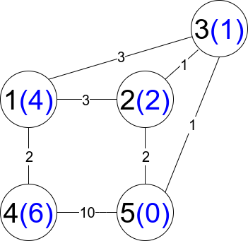
Input: n = 5, edges = [[1,2,3],[1,3,3],[2,3,1],[1,4,2],[5,2,2],[3,5,1],[5,4,10]]
Output: 3
Explanation: Each circle contains the node number in black and its distanceToLastNode value in blue. The three restricted paths are:
1) 1 --> 2 --> 5
2) 1 --> 2 --> 3 --> 5
3) 1 --> 3 --> 5

Example 2:

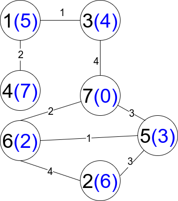
Input: n = 7, edges = [[1,3,1],[4,1,2],[7,3,4],[2,5,3],[5,6,1],[6,7,2],[7,5,3],[2,6,4]]
Output: 1
Explanation: Each circle contains the node number in black and its distanceToLastNode value in blue. The only restricted path is 1 --> 3 --> 7.


Constraints:

  • 1 <= n <= 2 * 104
  • n - 1 <= edges.length <= 4 * 104
  • edges[i].length == 3
  • 1 <= ui, vi <= n
  • ui != vi
  • 1 <= weighti <= 105
  • There is at most one edge between any two nodes.
  • There is at least one path between any two nodes.

Solution Explanation for LeetCode 1786: Number of Restricted Paths From First to Last Node

This problem asks to find the number of restricted paths from node 1 to node n in a weighted directed graph. A restricted path is a path where the shortest distance from each node to the last node (node n) strictly decreases as we move along the path.

The solution uses a combination of Dijkstra's algorithm and dynamic programming (DP) with topological sort implicitly handled by the sorting.

1. Finding Shortest Distances:

First, we use Dijkstra's algorithm to find the shortest distance from each node to the destination node (node n). Dijkstra's algorithm efficiently finds the shortest paths from a single source node to all other nodes in a weighted graph. We use a min-heap priority queue for efficiency.

  • A dist array stores the shortest distance from each node to node n. Initially, dist[n] = 0, and all other distances are set to infinity.

  • The algorithm iteratively selects the node with the smallest distance from the heap and updates the distances of its neighbors if a shorter path is found.

2. Dynamic Programming with Topological Sort (Implicit):

After obtaining shortest distances, we use dynamic programming to count restricted paths. We create a f array where f[i] represents the number of restricted paths from node i to node n.

  • We sort the nodes in ascending order of their shortest distances to node n (dist values). This implicitly handles the topological sort necessary for DP. Processing nodes in this order ensures that when calculating f[i], we've already computed f[j] for all nodes j that are reachable from i and have shorter distances to n (i.e., dist[i] > dist[j]).

  • For each node i, we iterate through its neighbors j. If dist[i] > dist[j] (which satisfies the restricted path condition), we add f[j] to f[i], taking the modulo 10^9 + 7 to avoid integer overflow. f[n] is initialized to 1 because there's one path from node n to itself.

3. Time Complexity Analysis:

  • Dijkstra's Algorithm: The time complexity of Dijkstra's algorithm using a min-heap is O(E log V), where E is the number of edges and V is the number of vertices (nodes).

  • Dynamic Programming: The sorting step takes O(V log V) time. The DP step iterates through all edges, so it takes O(E) time.

  • Overall: The dominant factor is Dijkstra's algorithm, so the overall time complexity is O(E log V).

4. Space Complexity Analysis:

  • dist array: O(V) space

  • g (adjacency list): O(E) space

  • f array: O(V) space

  • Priority Queue: O(V) in the worst case

  • Overall: The space complexity is O(E + V).

Code Examples (Python):

The Python code efficiently implements the described algorithm. The @cache decorator in the first solution and the f array in the second solution both optimize by storing and reusing already calculated results, thus improving efficiency, though the second solution avoids recursion and might be slightly more efficient for very large graphs. Both solutions share the same asymptotic complexities.

Other Languages:

The provided code also includes Java and C++ implementations. They follow the same logic and have similar time and space complexities. The Go implementation uses a custom heap structure for the priority queue. All implementations carefully handle modulo operations to avoid integer overflow issues.