{x}
blog image

Minimum Cost Homecoming of a Robot in a Grid

There is an m x n grid, where (0, 0) is the top-left cell and (m - 1, n - 1) is the bottom-right cell. You are given an integer array startPos where startPos = [startrow, startcol] indicates that initially, a robot is at the cell (startrow, startcol). You are also given an integer array homePos where homePos = [homerow, homecol] indicates that its home is at the cell (homerow, homecol).

The robot needs to go to its home. It can move one cell in four directions: left, right, up, or down, and it can not move outside the boundary. Every move incurs some cost. You are further given two 0-indexed integer arrays: rowCosts of length m and colCosts of length n.

  • If the robot moves up or down into a cell whose row is r, then this move costs rowCosts[r].
  • If the robot moves left or right into a cell whose column is c, then this move costs colCosts[c].

Return the minimum total cost for this robot to return home.


Example 1:

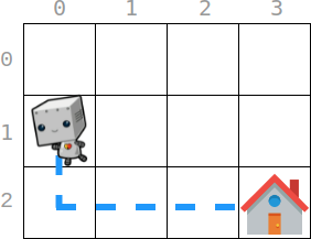
Input: startPos = [1, 0], homePos = [2, 3], rowCosts = [5, 4, 3], colCosts = [8, 2, 6, 7]
Output: 18
Explanation: One optimal path is that:
Starting from (1, 0)
-> It goes down to (2, 0). This move costs rowCosts[2] = 3.
-> It goes right to (2, 1). This move costs colCosts[1] = 2.
-> It goes right to (2, 2). This move costs colCosts[2] = 6.
-> It goes right to (2, 3). This move costs colCosts[3] = 7.
The total cost is 3 + 2 + 6 + 7 = 18

Example 2:

Input: startPos = [0, 0], homePos = [0, 0], rowCosts = [5], colCosts = [26]
Output: 0
Explanation: The robot is already at its home. Since no moves occur, the total cost is 0.


Constraints:

  • m == rowCosts.length
  • n == colCosts.length
  • 1 <= m, n <= 105
  • 0 <= rowCosts[r], colCosts[c] <= 104
  • startPos.length == 2
  • homePos.length == 2
  • 0 <= startrow, homerow < m
  • 0 <= startcol, homecol < n

Solution Explanation for Minimum Cost Homecoming of a Robot in a Grid

This problem involves finding the minimum cost for a robot to travel from a starting position to its home position in a grid. The robot can move up, down, left, or right, with the cost of each move depending on the row or column.

Approach:

The optimal approach is a greedy one. Since the cost of moving in a row or column only depends on the row or column index, respectively, the most efficient way to reach the home position is to move directly to it along the rows and then along the columns (or vice versa). This avoids unnecessary detours. We calculate the cost of moving in each direction separately and sum them up to get the total minimum cost.

Algorithm:

  1. Initialize: Start with a total cost ans initialized to 0.
  2. Row Movement: Calculate the cost of moving from the starting row to the home row.
    • If the starting row is less than the home row, iterate through rowCosts from startRow + 1 to homeRow (inclusive) and add each cost to ans.
    • If the starting row is greater than the home row, iterate through rowCosts from homeRow to startRow (inclusive) and add each cost to ans.
  3. Column Movement: Calculate the cost of moving from the starting column to the home column.
    • If the starting column is less than the home column, iterate through colCosts from startCol + 1 to homeCol (inclusive) and add each cost to ans.
    • If the starting column is greater than the home column, iterate through colCosts from homeCol to startCol (inclusive) and add each cost to ans.
  4. Return: Return the final calculated ans as the minimum total cost.

Time and Space Complexity:

  • Time Complexity: O(m + n), where m is the number of rows and n is the number of columns. This is because we iterate through at most the entire rowCosts array and the entire colCosts array once.
  • Space Complexity: O(1). The algorithm uses only a constant amount of extra space to store variables.

Code Implementation:

The code implementations in Python, Java, C++, and Go follow the algorithm described above. The Python and C++ versions use the sum() function to efficiently add up the elements of the relevant slices of the cost arrays. The Go version uses a helper function sum to achieve the same. The Java version iterates explicitly. All versions achieve the same optimal time complexity.

Example (Python):

class Solution:
    def minCost(
        self,
        startPos: List[int],
        homePos: List[int],
        rowCosts: List[int],
        colCosts: List[int],
    ) -> int:
        startRow, startCol = startPos
        homeRow, homeCol = homePos
        ans = 0
        if startRow < homeRow:
            ans += sum(rowCosts[startRow + 1:homeRow + 1])
        else:
            ans += sum(rowCosts[homeRow:startRow])
        if startCol < homeCol:
            ans += sum(colCosts[startCol + 1:homeCol + 1])
        else:
            ans += sum(colCosts[homeCol:startCol])
        return ans
 

The other languages have similar implementations, reflecting the same algorithm with minor syntactic differences. The choice of language does not impact the fundamental time or space complexity.