Given the root
of a binary tree, return the maximum width of the given tree.
The maximum width of a tree is the maximum width among all levels.
The width of one level is defined as the length between the end-nodes (the leftmost and rightmost non-null nodes), where the null nodes between the end-nodes that would be present in a complete binary tree extending down to that level are also counted into the length calculation.
It is guaranteed that the answer will in the range of a 32-bit signed integer.
Example 1:
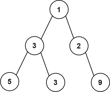
Input: root = [1,3,2,5,3,null,9] Output: 4 Explanation: The maximum width exists in the third level with length 4 (5,3,null,9).
Example 2:
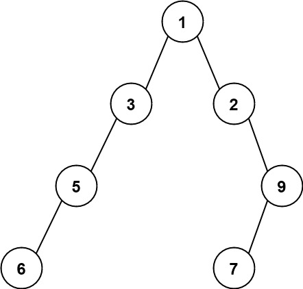
Input: root = [1,3,2,5,null,null,9,6,null,7] Output: 7 Explanation: The maximum width exists in the fourth level with length 7 (6,null,null,null,null,null,7).
Example 3:
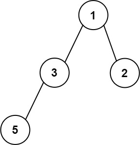
Input: root = [1,3,2,5] Output: 2 Explanation: The maximum width exists in the second level with length 2 (3,2).
Constraints:
[1, 3000]
.-100 <= Node.val <= 100
This problem asks to find the maximum width of a binary tree. The width of a level is the length between the leftmost and rightmost non-null nodes, including null nodes between them.
This approach uses BFS to traverse the tree level by level. We assign each node a unique index based on its position in the level. The leftmost node at each level gets index 1, the next node gets index 2, and so on. We use a queue to store pairs of (node, index).
Algorithm:
q
containing the root node with index 1. Initialize max_width
to 0.max_width
to the maximum of max_width
and the difference between the last node's index and the first node's index plus 1. This represents the width of the current level.2 * index
.2 * index + 1
.max_width
.Time Complexity: O(N), where N is the number of nodes in the tree. Each node is visited and processed once.
Space Complexity: O(W), where W is the maximum width of the tree. In the worst case (a complete binary tree), W can be proportional to N.
This approach uses DFS to traverse the tree. It maintains a list t
to store the index of the leftmost node at each level.
Algorithm:
t
and set ans
(maximum width) to 1.t
, append the index i
to t
.ans
to the maximum of ans
and i - t[depth] + 1
.i * 2
and i * 2 + 1
respectively) and depth.ans
.Time Complexity: O(N), where N is the number of nodes in the tree. Each node is visited and processed once.
Space Complexity: O(H), where H is the height of the tree. This is due to the recursive call stack in the worst case, and the size of t
which is at most H.
Approach 1 (BFS):
from collections import deque
class Solution:
def widthOfBinaryTree(self, root):
if not root:
return 0
q = deque([(root, 1)])
max_width = 0
while q:
max_width = max(max_width, q[-1][1] - q[0][1] + 1)
for _ in range(len(q)):
node, index = q.popleft()
if node.left:
q.append((node.left, index * 2))
if node.right:
q.append((node.right, index * 2 + 1))
return max_width
Approach 2 (DFS):
class Solution:
def widthOfBinaryTree(self, root):
self.ans = 1
self.t = []
self.dfs(root, 0, 1)
return self.ans
def dfs(self, root, depth, i):
if not root:
return
if len(self.t) == depth:
self.t.append(i)
else:
self.ans = max(self.ans, i - self.t[depth] + 1)
self.dfs(root.left, depth + 1, i * 2)
self.dfs(root.right, depth + 1, i * 2 + 1)
Both approaches have the same time complexity, but the BFS approach might be slightly more space-efficient for very wide trees because the DFS approach's space complexity depends on the height of the tree. The BFS approach's space complexity depends on the maximum width of the tree. For balanced trees, both have similar space complexity. For skewed trees, BFS can use significantly less space.