{x}
blog image

Count Good Nodes in Binary Tree

Given a binary tree root, a node X in the tree is named good if in the path from root to X there are no nodes with a value greater than X.

Return the number of good nodes in the binary tree.


Example 1:

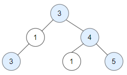
Input: root = [3,1,4,3,null,1,5]
Output: 4
Explanation: Nodes in blue are good.
Root Node (3) is always a good node.
Node 4 -> (3,4) is the maximum value in the path starting from the root.
Node 5 -> (3,4,5) is the maximum value in the path
Node 3 -> (3,1,3) is the maximum value in the path.

Example 2:

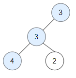
Input: root = [3,3,null,4,2]
Output: 3
Explanation: Node 2 -> (3, 3, 2) is not good, because "3" is higher than it.

Example 3:

Input: root = [1]
Output: 1
Explanation: Root is considered as good.


Constraints:

  • The number of nodes in the binary tree is in the range [1, 10^5].
  • Each node's value is between [-10^4, 10^4].

Solution Explanation:

This problem asks to count the number of "good nodes" in a binary tree. A node is considered good if there are no nodes with a value greater than its value on the path from the root to that node. The solution uses Depth-First Search (DFS) to efficiently traverse the tree and count these good nodes.

Approach:

The core idea is to perform a depth-first traversal of the binary tree. For each node visited, we keep track of the maximum value encountered so far on the path from the root. If the current node's value is greater than or equal to this maximum value, it's a "good node," and we increment the count. Otherwise, it's not a good node.

The DFS function recursively explores the left and right subtrees, updating the maximum value along the way.

Time Complexity Analysis:

The DFS approach visits each node in the binary tree exactly once. Therefore, the time complexity is O(N), where N is the number of nodes in the tree. This is linear time complexity.

Space Complexity Analysis:

The space complexity depends on the depth of the recursion. In the worst-case scenario (a skewed tree), the recursion depth is equal to the height of the tree, which can be O(N) in a completely skewed tree. In a balanced tree, the height is O(log N). Therefore, the space complexity is O(H), where H is the height of the tree. In the worst case, this becomes O(N), while in a balanced tree, it's O(log N). This is due to the recursive call stack used during the DFS traversal.

Code Explanation (Python):

class Solution:
    def goodNodes(self, root: TreeNode) -> int:
        def dfs(root: TreeNode, mx: int):
            if root is None:
                return
            nonlocal ans
            if mx <= root.val:  #Check if current node value is >= max value seen so far
                ans += 1      #Increment count if it's a good node
                mx = root.val #Update max value
            dfs(root.left, mx)  #Recursive call for left subtree
            dfs(root.right, mx) #Recursive call for right subtree
 
        ans = 0
        dfs(root, -1000000) #Initialize with a very small value for max.
        return ans

The Python code clearly implements the described DFS approach. The dfs function recursively traverses the tree, keeping track of the maximum value (mx) encountered on the path. The nonlocal ans keyword is used to modify the ans variable defined in the outer scope. The initial mx value is set to a very small number to ensure that the root node is always considered a good node.

The other languages (Java, C++, Go, TypeScript) follow a very similar structure and logic, differing only in syntax. They all achieve the same O(N) time and O(H) space complexity.