There is an m x n
matrix that is initialized to all 0
's. There is also a 2D array indices
where each indices[i] = [ri, ci]
represents a 0-indexed location to perform some increment operations on the matrix.
For each location indices[i]
, do both of the following:
ri
.ci
.Given m
, n
, and indices
, return the number of odd-valued cells in the matrix after applying the increment to all locations in indices
.
Example 1:
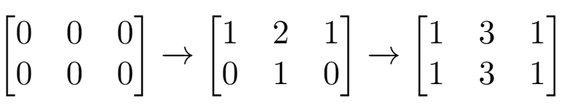
Input: m = 2, n = 3, indices = [[0,1],[1,1]] Output: 6 Explanation: Initial matrix = [[0,0,0],[0,0,0]]. After applying first increment it becomes [[1,2,1],[0,1,0]]. The final matrix is [[1,3,1],[1,3,1]], which contains 6 odd numbers.
Example 2:
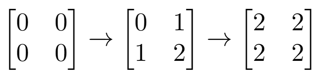
Input: m = 2, n = 2, indices = [[1,1],[0,0]] Output: 0 Explanation: Final matrix = [[2,2],[2,2]]. There are no odd numbers in the final matrix.
Constraints:
1 <= m, n <= 50
1 <= indices.length <= 100
0 <= ri < m
0 <= ci < n
Follow up: Could you solve this in O(n + m + indices.length)
time with only O(n + m)
extra space?
This problem involves a matrix initialized with zeros and a series of operations that increment rows and columns based on given indices. The goal is to efficiently count the number of cells with odd values after all operations.
Core Idea: Instead of explicitly creating and modifying the matrix (which would be inefficient for large matrices), we can track the number of times each row and column is incremented. The final value of a cell (i, j) will be the sum of increments to row i and column j.
Three Approaches:
The problem can be solved in three ways, each with different time and space complexities:
1. Simulation:
indices
, m is the number of rows, and n is the number of columns. The dominant factor is the nested loops for incrementing and counting.2. Space Optimization:
row
and col
. row[i]
stores the number of times row i
is incremented, and similarly for columns. The value of a cell (i, j) is then row[i] + col[j]
. We iterate through all possible cell indices and count odd values.row
and col
takes O(m+n), the loop for increments takes O(k), and the final counting loop takes O(mn).row
and col
arrays.3. Mathematical Optimization:
row[i]
and col[j]
is odd. We count odd rows (cnt1
) and odd columns (cnt2
). The number of odd cells is then cnt1 * (n - cnt2) + cnt2 * (m - cnt1)
.row
and col
arrays.Code Examples (Python):
Approach 1 (Simulation):
class Solution:
def oddCells(self, m: int, n: int, indices: List[List[int]]) -> int:
matrix = [[0] * n for _ in range(m)]
for r, c in indices:
for i in range(m):
matrix[i][c] += 1
for j in range(n):
matrix[r][j] += 1
count = 0
for row in matrix:
for cell in row:
if cell % 2 != 0:
count += 1
return count
Approach 2 (Space Optimization):
class Solution:
def oddCells(self, m: int, n: int, indices: List[List[int]]) -> int:
row_inc = [0] * m
col_inc = [0] * n
for r, c in indices:
row_inc[r] += 1
col_inc[c] += 1
count = 0
for i in range(m):
for j in range(n):
if (row_inc[i] + col_inc[j]) % 2 != 0:
count += 1
return count
Approach 3 (Mathematical Optimization):
class Solution:
def oddCells(self, m: int, n: int, indices: List[List[int]]) -> int:
row_inc = [0] * m
col_inc = [0] * n
for r, c in indices:
row_inc[r] += 1
col_inc[c] += 1
odd_rows = sum(1 for x in row_inc if x % 2 != 0)
odd_cols = sum(1 for x in col_inc if x % 2 != 0)
return odd_rows * (n - odd_cols) + odd_cols * (m - odd_rows)
The mathematical optimization (Approach 3) provides the best time complexity, making it the most efficient solution for large input sizes. The other approaches are provided for comparison and illustrative purposes. The space complexity is similar for approaches 2 and 3. Approach 1 is significantly less efficient in both time and space for large inputs.