A matrix diagonal is a diagonal line of cells starting from some cell in either the topmost row or leftmost column and going in the bottom-right direction until reaching the matrix's end. For example, the matrix diagonal starting from mat[2][0]
, where mat
is a 6 x 3
matrix, includes cells mat[2][0]
, mat[3][1]
, and mat[4][2]
.
Given an m x n
matrix mat
of integers, sort each matrix diagonal in ascending order and return the resulting matrix.
Example 1:
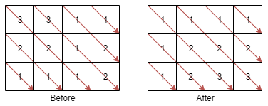
Input: mat = [[3,3,1,1],[2,2,1,2],[1,1,1,2]] Output: [[1,1,1,1],[1,2,2,2],[1,2,3,3]]
Example 2:
Input: mat = [[11,25,66,1,69,7],[23,55,17,45,15,52],[75,31,36,44,58,8],[22,27,33,25,68,4],[84,28,14,11,5,50]] Output: [[5,17,4,1,52,7],[11,11,25,45,8,69],[14,23,25,44,58,15],[22,27,31,36,50,66],[84,28,75,33,55,68]]
Constraints:
m == mat.length
n == mat[i].length
1 <= m, n <= 100
1 <= mat[i][j] <= 100
This problem requires sorting the elements along each diagonal of a given matrix. The solution leverages the observation that elements on the same diagonal share a consistent relationship between their row and column indices.
Core Idea:
Diagonal Identification: Elements on the same diagonal have a constant difference between their column index and row index ( j - i
). However, to avoid negative indices, we use m - i + j
where m
is the number of rows, ensuring a positive index for each diagonal. This value serves as the unique identifier for each diagonal.
Grouping by Diagonal: We use a list (or array) to group elements based on their diagonal identifier. Each index in the list represents a diagonal, and the elements at that index are the numbers belonging to that diagonal.
Sorting Diagonals: We sort the elements within each diagonal in ascending order.
Reconstruction: We iterate through the matrix again. This time, we reconstruct the matrix by placing the sorted elements back into their original positions based on their diagonal. The sorted values are removed from the grouping arrays as we reconstruct the matrix.
Time Complexity Analysis:
m x n
matrix takes O(mn) time.min(m, n)
. Therefore, the total sorting time is O(mn log(min(m, n))).Therefore, the overall time complexity is dominated by the sorting step, resulting in O(mn log(min(m, n))).
Space Complexity Analysis:
The space complexity is determined by the size of the g
array (used for grouping diagonals), which stores all the matrix elements. In the worst-case scenario (a square matrix), it will store all mn
elements. Thus, the space complexity is O(mn).
Code Explanation (Python3):
class Solution:
def diagonalSort(self, mat: List[List[int]]) -> List[List[int]]:
m, n = len(mat), len(mat[0])
g = [[] for _ in range(m + n)] # Initialize a list to store elements of each diagonal
# Grouping elements by diagonal
for i, row in enumerate(mat):
for j, x in enumerate(row):
g[m - i + j].append(x)
# Sorting each diagonal
for e in g:
e.sort() # sorts in ascending order
# Reconstructing the matrix
for i in range(m):
for j in range(n):
mat[i][j] = g[m - i + j].pop(0) # Removes the first element (smallest)
return mat
The other language implementations follow a very similar structure, differing primarily in syntax and data structure usage (e.g., ArrayList
in Java, vector
in C++, slices in Go etc.). The fundamental algorithmic approach remains consistent across all implementations.