
Number Of Ways To Reconstruct A Tree
You are given an array pairs, where pairs[i] = [xi, yi], and:
- There are no duplicates.
xi < yi
Let ways be the number of rooted trees that satisfy the following conditions:
- The tree consists of nodes whose values appeared in
pairs. - A pair
[xi, yi]exists inpairsif and only ifxiis an ancestor ofyioryiis an ancestor ofxi. - Note: the tree does not have to be a binary tree.
Two ways are considered to be different if there is at least one node that has different parents in both ways.
Return:
0ifways == 01ifways == 12ifways > 1
A rooted tree is a tree that has a single root node, and all edges are oriented to be outgoing from the root.
An ancestor of a node is any node on the path from the root to that node (excluding the node itself). The root has no ancestors.
Example 1:
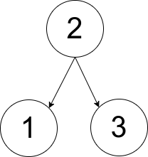
Input: pairs = [[1,2],[2,3]]
Output: 1
Explanation: There is exactly one valid rooted tree, which is shown in the above figure.
Example 2:
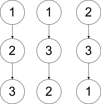
Input: pairs = [[1,2],[2,3],[1,3]]
Output: 2
Explanation: There are multiple valid rooted trees. Three of them are shown in the above figures.
Example 3:
Input: pairs = [[1,2],[2,3],[2,4],[1,5]]
Output: 0
Explanation: There are no valid rooted trees.
Constraints:
1 <= pairs.length <= 1051 <= xi < yi <= 500- The elements in
pairsare unique.
On This Page
Also Explore
DSA Questions
Count Good Meals
DSA Questions
Ways to Split Array Into Three Subarrays
DSA Questions
Minimum Operations to Make a Subsequence
DSA Questions
Sum Of Special Evenly-Spaced Elements In Array
DSA Questions
Count Apples and Oranges
DSA Questions
Calculate Money in Leetcode Bank
DSA Questions
Maximum Score From Removing Substrings
DSA Questions
Number Of Ways To Reconstruct A Tree
DSA Questions
Decode XORed Array
DSA Questions
Swapping Nodes in a Linked List
DSA Questions
Minimize Hamming Distance After Swap Operations
DSA Questions
Find Minimum Time to Finish All Jobs
DSA Questions
Checking Existence of Edge Length Limited Paths II
DSA Questions
Tuple with Same Product
DSA Questions