{x}
blog image

Number of Provinces

There are n cities. Some of them are connected, while some are not. If city a is connected directly with city b, and city b is connected directly with city c, then city a is connected indirectly with city c.

A province is a group of directly or indirectly connected cities and no other cities outside of the group.

You are given an n x n matrix isConnected where isConnected[i][j] = 1 if the ith city and the jth city are directly connected, and isConnected[i][j] = 0 otherwise.

Return the total number of provinces.


Example 1:

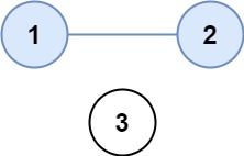
Input: isConnected = [[1,1,0],[1,1,0],[0,0,1]]
Output: 2

Example 2:

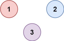
Input: isConnected = [[1,0,0],[0,1,0],[0,0,1]]
Output: 3


Constraints:

  • 1 <= n <= 200
  • n == isConnected.length
  • n == isConnected[i].length
  • isConnected[i][j] is 1 or 0.
  • isConnected[i][i] == 1
  • isConnected[i][j] == isConnected[j][i]

547. Number of Provinces

Description

The problem asks to find the number of provinces in a given graph represented by an adjacency matrix isConnected. A province is a group of directly or indirectly connected cities. Two cities are directly connected if isConnected[i][j] == 1.

Solutions

Two common approaches to solve this problem are Depth-First Search (DFS) and Union-Find.

Solution 1: Depth-First Search (DFS)

This approach uses DFS to traverse the graph and identify connected components.

Algorithm:

  1. Initialization: Create a boolean array vis of size n (number of cities), initialized to false. This array tracks visited cities. Initialize a counter ans to 0, representing the number of provinces.

  2. Iteration: Iterate through each city i from 0 to n-1.

  3. DFS Check: If vis[i] is false (city i is not visited), it means a new province is found. Increment ans. Call a recursive DFS function starting from city i.

  4. DFS Function: The DFS function dfs(i) marks vis[i] as true. Then, it iterates through the neighbors of city i (cities j where isConnected[i][j] == 1). If a neighbor j is not visited (vis[j] is false), it recursively calls dfs(j) to explore that neighbor's connected components.

Time Complexity: O(N^2), where N is the number of cities. This is because we visit each city and its neighbors once. In the worst case, we might traverse all the edges of the graph.

Space Complexity: O(N) to store the vis array. The recursive call stack in DFS also contributes to space complexity, but it's bounded by the height of the graph, which is at most N in this case.

Code (Python):

class Solution:
    def findCircleNum(self, isConnected: List[List[int]]) -> int:
        n = len(isConnected)
        vis = [False] * n
        ans = 0
 
        def dfs(i: int):
            vis[i] = True
            for j in range(n):
                if isConnected[i][j] and not vis[j]:
                    dfs(j)
 
        for i in range(n):
            if not vis[i]:
                dfs(i)
                ans += 1
        return ans
 

Similar code can be written in other languages like Java, C++, JavaScript, etc., following the same algorithm.

Solution 2: Union-Find

Union-find is a disjoint-set data structure that efficiently tracks connected components.

Algorithm:

  1. Initialization: Create a parent array p of size n, where initially p[i] = i (each city is its own parent, representing separate components). Initialize a count ans to n (initially, each city is a separate province).

  2. Iteration: Iterate through the isConnected matrix.

  3. Union: If isConnected[i][j] == 1, find the root parents of i and j using a find function (with path compression for optimization). If the roots are different, it means i and j belong to different components. Perform a union operation by setting p[root_of_i] = root_of_j, merging the components. Decrement ans because we've merged two provinces.

  4. Find Function: The find function recursively finds the root parent of a node, applying path compression to optimize subsequent find operations.

Time Complexity: O(N^2 * α(N)), where α(N) is the inverse Ackermann function, which grows extremely slowly and is practically a constant. The O(N^2) factor comes from iterating through the adjacency matrix. Path compression significantly improves the performance of Union-Find.

Space Complexity: O(N) to store the p array.

Code (Python):

class Solution:
    def findCircleNum(self, isConnected: List[List[int]]) -> int:
        n = len(isConnected)
        p = list(range(n))
        ans = n
 
        def find(x: int) -> int:
            if p[x] != x:
                p[x] = find(p[x])  # Path compression
            return p[x]
 
        for i in range(n):
            for j in range(i + 1, n):
                if isConnected[i][j]:
                    root_i = find(i)
                    root_j = find(j)
                    if root_i != root_j:
                        p[root_i] = root_j
                        ans -= 1
        return ans

Again, similar code can be written in other languages.

Choosing between DFS and Union-Find:

For this specific problem, DFS is often slightly simpler to implement. Union-Find's advantage becomes more apparent in problems involving more complex queries on connected components. The asymptotic time complexities are similar in practice, with Union-Find possibly having a slight edge due to path compression.