{x}
blog image

01 Matrix

Given an m x n binary matrix mat, return the distance of the nearest 0 for each cell.

The distance between two cells sharing a common edge is 1.


Example 1:

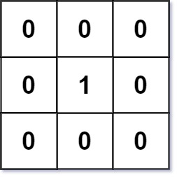
Input: mat = [[0,0,0],[0,1,0],[0,0,0]]
Output: [[0,0,0],[0,1,0],[0,0,0]]

Example 2:

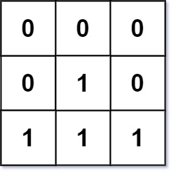
Input: mat = [[0,0,0],[0,1,0],[1,1,1]]
Output: [[0,0,0],[0,1,0],[1,2,1]]


Constraints:

  • m == mat.length
  • n == mat[i].length
  • 1 <= m, n <= 104
  • 1 <= m * n <= 104
  • mat[i][j] is either 0 or 1.
  • There is at least one 0 in mat.


Note: This question is the same as 1765: https://leetcode.com/problems/map-of-highest-peak/

Solution Explanation: 01 Matrix

This problem asks to find the shortest distance from each cell in a binary matrix to the nearest 0. The most efficient approach is using Breadth-First Search (BFS).

Algorithm:

  1. Initialization:

    • Create a result matrix ans of the same dimensions as the input mat, filled with -1 (representing infinity, as we haven't reached these cells yet).
    • Create a queue q to store coordinates of cells containing 0. Add all coordinates of 0s from mat to q. Set the corresponding values in ans to 0.
  2. BFS Traversal:

    • While the queue q is not empty:
      • Dequeue a cell (row, col) from q.
      • Explore its four neighboring cells (up, down, left, right).
      • For each neighbor:
        • If the neighbor is within the matrix bounds AND its value in ans is still -1 (meaning it hasn't been visited):
          • Update the neighbor's value in ans to the distance from the nearest 0 (distance from the current cell + 1).
          • Enqueue the neighbor's coordinates into q.
  3. Return:

    • Return the ans matrix.

Time Complexity: O(M*N), where M and N are the dimensions of the matrix. Each cell is visited and processed at most once.

Space Complexity: O(M*N) in the worst case, which is when the queue holds all cells in the matrix (when all cells are 1s except for one 0).

Code Examples:

The provided code snippets in Python, Java, C++, Go, TypeScript, and Rust all implement the BFS algorithm. They differ slightly in syntax and data structures, but the core logic remains the same. Let's analyze a representative example (Python):

from collections import deque
 
class Solution:
    def updateMatrix(self, mat: List[List[int]]) -> List[List[int]]:
        m, n = len(mat), len(mat[0])
        ans = [[-1] * n for _ in range(m)]  # Initialize with -1
        q = deque()
 
        # Add all 0s to the queue
        for i in range(m):
            for j in range(n):
                if mat[i][j] == 0:
                    ans[i][j] = 0
                    q.append((i, j))
 
        # BFS traversal
        while q:
            i, j = q.popleft()
            for x, y in [(i+1, j), (i-1, j), (i, j+1), (i, j-1)]: # Neighbors
                if 0 <= x < m and 0 <= y < n and ans[x][y] == -1:
                    ans[x][y] = ans[i][j] + 1
                    q.append((x, y))
 
        return ans
 

This Python code effectively demonstrates the BFS approach. The deque from the collections module is used as a queue for optimal performance in enqueue and dequeue operations. The nested loops efficiently add all initial 0s. The inner loop iterates over the four neighboring cells, ensuring only valid and unvisited cells are processed and added to the queue.

The other language implementations follow the same algorithmic steps, but with language-specific syntax and data structure choices. The time and space complexity remains consistent across all implementations.