You are given an image represented by an m x n
grid of integers image
, where image[i][j]
represents the pixel value of the image. You are also given three integers sr
, sc
, and color
. Your task is to perform a flood fill on the image starting from the pixel image[sr][sc]
.
To perform a flood fill:
color
.Return the modified image after performing the flood fill.
Example 1:
Input: image = [[1,1,1],[1,1,0],[1,0,1]], sr = 1, sc = 1, color = 2
Output: [[2,2,2],[2,2,0],[2,0,1]]
Explanation:
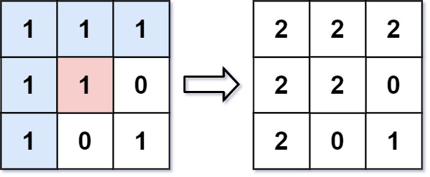
From the center of the image with position (sr, sc) = (1, 1)
(i.e., the red pixel), all pixels connected by a path of the same color as the starting pixel (i.e., the blue pixels) are colored with the new color.
Note the bottom corner is not colored 2, because it is not horizontally or vertically connected to the starting pixel.
Example 2:
Input: image = [[0,0,0],[0,0,0]], sr = 0, sc = 0, color = 0
Output: [[0,0,0],[0,0,0]]
Explanation:
The starting pixel is already colored with 0, which is the same as the target color. Therefore, no changes are made to the image.
Constraints:
m == image.length
n == image[i].length
1 <= m, n <= 50
0 <= image[i][j], color < 216
0 <= sr < m
0 <= sc < n
The Flood Fill algorithm is used to replace a connected component of a specified color with a new color. This problem presents a grid (image) where each cell represents a pixel with a certain color. We need to change the color of a connected component starting from a given pixel (sr, sc) to a new color.
Approaches:
Two common approaches exist to solve this problem: Depth-First Search (DFS) and Breadth-First Search (BFS). Both methods traverse the connected component, replacing the original color with the new color.
1. Depth-First Search (DFS) Approach:
DFS uses recursion to explore the connected component. It starts at the given pixel and recursively visits all adjacent pixels with the same color as the starting pixel.
Algorithm:
dfs(i, j)
that takes the row and column index as input.dfs
for the adjacent pixels (up, down, left, right).dfs(sr, sc)
to start the process at the given pixel.Time Complexity: O(M*N), where M and N are the dimensions of the image. In the worst case, we visit every pixel.
Space Complexity: O(M*N) in the worst-case scenario due to the recursive call stack. In the average case, it is less but still can be significant for large images.
2. Breadth-First Search (BFS) Approach:
BFS uses a queue to explore the connected component level by level. It starts at the given pixel and adds its neighbors to the queue. It then processes the pixels from the queue one by one.
Algorithm:
q
and add the given pixel (sr, sc) to it.Time Complexity: O(M*N), same as DFS.
Space Complexity: O(M*N) in the worst case, where the queue might contain all pixels. Generally considered to have better space efficiency than DFS for very large connected components.
Code Examples (Python):
DFS:
def floodFill(image, sr, sc, color):
m, n = len(image), len(image[0])
original_color = image[sr][sc]
def dfs(i, j):
if (0 <= i < m and 0 <= j < n and image[i][j] == original_color and image[i][j] != color):
image[i][j] = color
dfs(i + 1, j)
dfs(i - 1, j)
dfs(i, j + 1)
dfs(i, j - 1)
dfs(sr, sc)
return image
BFS:
from collections import deque
def floodFill(image, sr, sc, color):
m, n = len(image), len(image[0])
original_color = image[sr][sc]
q = deque([(sr, sc)])
while q:
i, j = q.popleft()
if 0 <= i < m and 0 <= j < n and image[i][j] == original_color and image[i][j] != color:
image[i][j] = color
q.append((i + 1, j))
q.append((i - 1, j))
q.append((i, j + 1))
q.append((i, j - 1))
return image
The provided code examples in other languages (Java, C++, Go, TypeScript, Rust) follow the same logic, either using DFS recursion or BFS with a queue. The choice between DFS and BFS often depends on the specific problem and memory constraints. For this problem, the difference in performance is usually negligible.