Given the root
of a binary tree, each node in the tree has a distinct value.
After deleting all nodes with a value in to_delete
, we are left with a forest (a disjoint union of trees).
Return the roots of the trees in the remaining forest. You may return the result in any order.
Example 1:
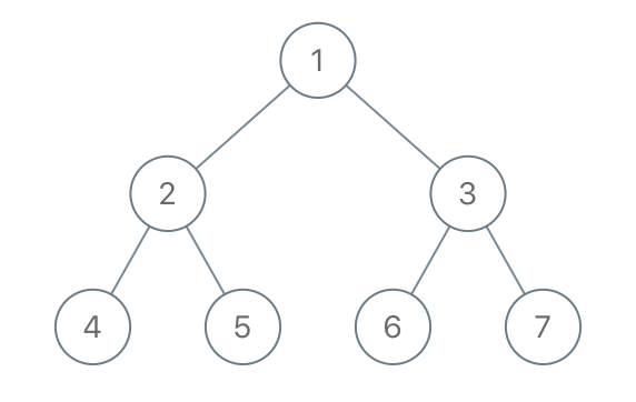
Input: root = [1,2,3,4,5,6,7], to_delete = [3,5] Output: [[1,2,null,4],[6],[7]]
Example 2:
Input: root = [1,2,4,null,3], to_delete = [3] Output: [[1,2,4]]
Constraints:
1000
.1
and 1000
.to_delete.length <= 1000
to_delete
contains distinct values between 1
and 1000
.The problem requires deleting nodes with specific values from a binary tree and returning the roots of the resulting forest (a collection of disjoint trees). The provided solutions leverage depth-first search (DFS) and breadth-first search (BFS) to efficiently achieve this.
This approach uses a recursive DFS strategy. The core idea is to traverse the tree, process each node, and rebuild the tree structure based on whether a node should be deleted.
Initialization: A set s
(or a boolean array in some implementations) is created to store the values of nodes to be deleted. This allows for O(1) lookup time when checking if a node should be deleted.
dfs(root)
Function: This recursive function performs the following:
root
is null
, it returns null
.dfs
on the left and right subtrees, updating root.left
and root.right
with the results.root.val
is in s
(node should be deleted), it checks if the left and right children are not null
. If they exist, they are added to the ans
list (representing the roots of the resulting forest) because they become the roots of new subtrees. The function then returns null
to remove the current node from the tree.root.val
is not in s
, the function returns root
, preserving the node in the tree.Main Function: The dfs
function is called on the root. If the returned value is not null
, it means the root node was not deleted, and it's added to ans
. Finally, ans
(containing the roots of the remaining trees) is returned.
Time Complexity: O(N), where N is the number of nodes in the tree. Each node is visited and processed exactly once.
Space Complexity: O(N) in the worst case due to the recursive call stack (depth of the tree) and the ans
list (in the worst case, all nodes except the deleted ones could become roots). The set s
uses O(K) space, where K is the number of nodes to delete; this is typically much smaller than N.
This approach uses an iterative BFS strategy. It processes the tree level by level, using a queue.
Initialization: Similar to DFS, a set del
is used to store the values of nodes to be deleted. A queue q
is initialized with the root node. The result list res
will hold the roots of the remaining trees.
Iteration: The while
loop iterates as long as the queue q
is not empty.
q
.qNext
queue, and if their values are in del
, the children are set to null
in the parent.del
, its left and right children (if not null
) are added to res
as new roots.qNext
becomes the new q
for the next iteration.Root Check: Finally, if the root node's value is not in del
, the root is added to res
.
Time Complexity: O(N), similar to DFS, as all nodes are processed once.
Space Complexity: O(W), where W is the maximum width of the tree. The queue can hold up to W nodes at any given time. In the worst-case scenario (a complete binary tree), W can be proportional to N, resulting in O(N) space complexity. The set del
uses O(K) space (as in DFS).
Both approaches provide correct solutions with a time complexity of O(N). The choice between DFS and BFS might depend on factors like the expected tree structure and memory constraints. DFS might be slightly more space-efficient for deeply nested trees, while BFS might be preferred for wide trees where the maximum width is significantly smaller than the number of nodes.