{x}
blog image

Cherry Pickup II

You are given a rows x cols matrix grid representing a field of cherries where grid[i][j] represents the number of cherries that you can collect from the (i, j) cell.

You have two robots that can collect cherries for you:

  • Robot #1 is located at the top-left corner (0, 0), and
  • Robot #2 is located at the top-right corner (0, cols - 1).

Return the maximum number of cherries collection using both robots by following the rules below:

  • From a cell (i, j), robots can move to cell (i + 1, j - 1), (i + 1, j), or (i + 1, j + 1).
  • When any robot passes through a cell, It picks up all cherries, and the cell becomes an empty cell.
  • When both robots stay in the same cell, only one takes the cherries.
  • Both robots cannot move outside of the grid at any moment.
  • Both robots should reach the bottom row in grid.


Example 1:

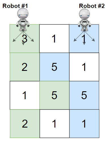
Input: grid = [[3,1,1],[2,5,1],[1,5,5],[2,1,1]]
Output: 24
Explanation: Path of robot #1 and #2 are described in color green and blue respectively.
Cherries taken by Robot #1, (3 + 2 + 5 + 2) = 12.
Cherries taken by Robot #2, (1 + 5 + 5 + 1) = 12.
Total of cherries: 12 + 12 = 24.

Example 2:

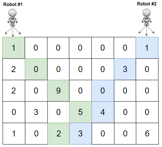
Input: grid = [[1,0,0,0,0,0,1],[2,0,0,0,0,3,0],[2,0,9,0,0,0,0],[0,3,0,5,4,0,0],[1,0,2,3,0,0,6]]
Output: 28
Explanation: Path of robot #1 and #2 are described in color green and blue respectively.
Cherries taken by Robot #1, (1 + 9 + 5 + 2) = 17.
Cherries taken by Robot #2, (1 + 3 + 4 + 3) = 11.
Total of cherries: 17 + 11 = 28.


Constraints:

  • rows == grid.length
  • cols == grid[i].length
  • 2 <= rows, cols <= 70
  • 0 <= grid[i][j] <= 100

Solution Explanation: Cherry Pickup II

This problem involves finding the maximum number of cherries two robots can collect while moving through a grid. Both robots start at the top row, one on the left and one on the right, and they must both reach the bottom row. They can move diagonally left, straight down, or diagonally right at each step. If they occupy the same cell, only one robot collects the cherries.

The optimal solution leverages dynamic programming. We'll explore two approaches: one with higher space complexity but potentially easier to understand, and another optimized for space.

Solution 1: Dynamic Programming (Higher Space Complexity)

This approach uses a 3D DP array f[i][j1][j2] to store the maximum cherries collected when:

  • i represents the current row.
  • j1 is the column index of robot 1.
  • j2 is the column index of robot 2.

State Transition:

The core idea is to build up the solution row by row. For each cell (i, j1, j2), we consider all possible previous positions (y1, y2) of the two robots in the previous row ( i-1). These positions are limited to the cells adjacent to (j1, j2) in the previous row, accounting for the possible movements. The transition equation is:

f[i][j1][j2] = max(f[i][j1][j2], f[i-1][y1][y2] + cherries_collected_in_row_i)

cherries_collected_in_row_i is calculated as:

  • grid[i][j1] + grid[i][j2] if j1 != j2 (robots in different cells).
  • grid[i][j1] if j1 == j2 (robots in same cell, only one collects).

Base Case:

f[0][0][n-1] = grid[0][0] + grid[0][n-1] (initial position of robots).

Final Result:

The maximum number of cherries is the maximum value in the last row of the DP array: max(f[m-1][j1][j2]) for all j1 and j2.

Time Complexity: O(m * n^3), where 'm' is the number of rows and 'n' is the number of columns. This comes from iterating through all possible states in the 3D DP array.

Space Complexity: O(m * n^2) to store the DP array f.

Solution 2: Dynamic Programming (Space Optimization)

The space complexity can be reduced to O(n^2) by using only two 2D arrays instead of a 3D array. We alternate between two arrays, f and g, updating one based on the other in each row. This eliminates the need to store the entire history of the DP array.

Time Complexity: O(m * n^3). The time complexity remains the same because we still need to explore all possible state transitions.

Space Complexity: O(n^2) to store the two 2D arrays f and g.

Code Examples (Python):

Solution 1 (Higher Space Complexity):

from itertools import product
 
def cherryPickup(grid):
    m, n = len(grid), len(grid[0])
    f = [[[-1] * n for _ in range(n)] for _ in range(m)]
    f[0][0][n - 1] = grid[0][0] + grid[0][n - 1]
    for i in range(1, m):
        for j1 in range(n):
            for j2 in range(n):
                x = grid[i][j1] + (0 if j1 == j2 else grid[i][j2])
                for y1 in range(max(0, j1 - 1), min(n, j1 + 2)):
                    for y2 in range(max(0, j2 - 1), min(n, j2 + 2)):
                        if f[i - 1][y1][y2] != -1:
                            f[i][j1][j2] = max(f[i][j1][j2], f[i - 1][y1][y2] + x)
    return max(f[-1][j1][j2] for j1, j2 in product(range(n), range(n)))
 

Solution 2 (Space Optimized):

from itertools import product
 
def cherryPickup(grid):
    m, n = len(grid), len(grid[0])
    f = [[-1] * n for _ in range(n)]
    g = [[-1] * n for _ in range(n)]
    f[0][n - 1] = grid[0][0] + grid[0][n - 1]
    for i in range(1, m):
        for j1 in range(n):
            for j2 in range(n):
                x = grid[i][j1] + (0 if j1 == j2 else grid[i][j2])
                for y1 in range(max(0, j1 - 1), min(n, j1 + 2)):
                    for y2 in range(max(0, j2 - 1), min(n, j2 + 2)):
                        if f[y1][y2] != -1:
                            g[j1][j2] = max(g[j1][j2], f[y1][y2] + x)
        f, g = g, f
        g = [[-1] * n for _ in range(n)] #Reset g for the next iteration
    return max(f[j1][j2] for j1, j2 in product(range(n), range(n)))
 

The code examples in other languages (Java, C++, Go, TypeScript) follow similar logic and structure as the Python examples, adapting syntax and data structures specific to each language. The core dynamic programming approach remains consistent.