There are n
cities connected by some number of flights. You are given an array flights
where flights[i] = [fromi, toi, pricei]
indicates that there is a flight from city fromi
to city toi
with cost pricei
.
You are also given three integers src
, dst
, and k
, return the cheapest price from src
to dst
with at most k
stops. If there is no such route, return -1
.
Example 1:
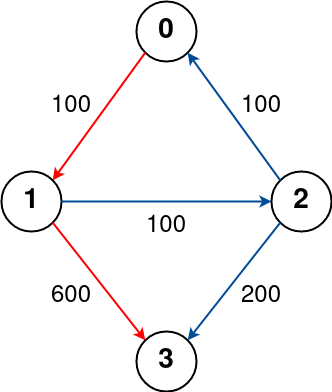
Input: n = 4, flights = [[0,1,100],[1,2,100],[2,0,100],[1,3,600],[2,3,200]], src = 0, dst = 3, k = 1 Output: 700 Explanation: The graph is shown above. The optimal path with at most 1 stop from city 0 to 3 is marked in red and has cost 100 + 600 = 700. Note that the path through cities [0,1,2,3] is cheaper but is invalid because it uses 2 stops.
Example 2:
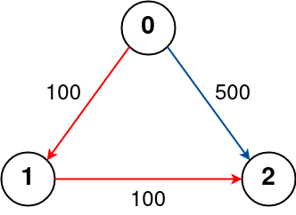
Input: n = 3, flights = [[0,1,100],[1,2,100],[0,2,500]], src = 0, dst = 2, k = 1 Output: 200 Explanation: The graph is shown above. The optimal path with at most 1 stop from city 0 to 2 is marked in red and has cost 100 + 100 = 200.
Example 3:
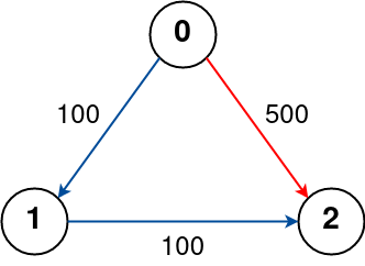
Input: n = 3, flights = [[0,1,100],[1,2,100],[0,2,500]], src = 0, dst = 2, k = 0 Output: 500 Explanation: The graph is shown above. The optimal path with no stops from city 0 to 2 is marked in red and has cost 500.
Constraints:
1 <= n <= 100
0 <= flights.length <= (n * (n - 1) / 2)
flights[i].length == 3
0 <= fromi, toi < n
fromi != toi
1 <= pricei <= 104
0 <= src, dst, k < n
src != dst
This problem asks to find the cheapest flight from a source city to a destination city with at most k stops. We can solve this using either Dynamic Programming or a variation of Breadth-First Search (BFS).
This approach iteratively relaxes edges in the flight graph. dist[i]
represents the minimum cost to reach city i
. We repeat this relaxation process k+1
times, representing up to k
stops.
Algorithm:
dist
of size n
, initialized to infinity except for the source city (src
), which is 0.k+1
times (representing 0 to k stops). In each iteration:
dist
array.flights
. For each flight (from, to, price)
, update dist[to]
with the minimum of its current value and backup[from] + price
. This represents the possibility of reaching city to
via city from
.dist[dst]
contains the minimum cost to reach the destination city. If it's still infinity, there's no path within k
stops.Time Complexity: O(k*E), where E is the number of flights. The outer loop iterates k+1 times, and the inner loop iterates through all flights.
Space Complexity: O(N), where N is the number of cities. We use an array dist
to store the minimum distances.
This recursive approach explores all possible paths from the source city to the destination city. Memoization is crucial to avoid redundant calculations.
Algorithm:
g
representing the flight graph.dfs(u, k)
:
u
is the destination, return 0 (cost is 0 to reach the destination).k
is 0 or less (no more stops allowed), return infinity.u
. For each flight (v, p)
to city v
with price p
:
dfs(v, k-1)
to find the minimum cost from v
to dst
with k-1
remaining stops.min(ans, dfs(v, k-1) + p)
.dfs(u, k)
in memo
to avoid redundant computations.dfs(src, k+1)
to start the search. Return -1 if the minimum cost is still infinity.Time Complexity: O(VE), where V is the number of vertices (cities) and E is the number of edges (flights). The worst-case scenario involves exploring all possible paths. Memoization significantly improves performance by reducing redundant calculations, although the worst-case complexity remains the same. Space Complexity: O(VK) due to memoization. We store the results for each city and number of stops.
Code Examples (Python, Java, C++, Go): The code examples provided in the original markdown are correct implementations of both approaches. The Python example uses the @cache
decorator for memoization, which makes it concise. The Java, C++, and Go solutions handle memoization manually. They also use adjacency matrices instead of adjacency lists, potentially leading to a larger space complexity if the graph is sparse. Using adjacency lists would typically be more efficient for sparse graphs.
The choice between the two approaches depends on the specific characteristics of the input data. For large graphs with many flights, the dynamic programming approach (Approach 1) might be more efficient due to its simpler iterative nature. For smaller graphs or cases where the maximum number of stops (k
) is relatively small, the memoized DFS (Approach 2) could also be efficient.