
All Ancestors of a Node in a Directed Acyclic Graph
You are given a positive integer n representing the number of nodes of a Directed Acyclic Graph (DAG). The nodes are numbered from 0 to n - 1 (inclusive).
You are also given a 2D integer array edges, where edges[i] = [fromi, toi] denotes that there is a unidirectional edge from fromi to toi in the graph.
Return a list answer, where answer[i] is the list of ancestors of the ith node, sorted in ascending order.
A node u is an ancestor of another node v if u can reach v via a set of edges.
Example 1:
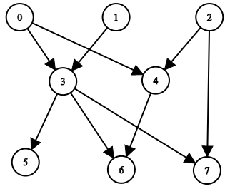
Input: n = 8, edgeList = [[0,3],[0,4],[1,3],[2,4],[2,7],[3,5],[3,6],[3,7],[4,6]]
Output: [[],[],[],[0,1],[0,2],[0,1,3],[0,1,2,3,4],[0,1,2,3]]
Explanation:
The above diagram represents the input graph.
- Nodes 0, 1, and 2 do not have any ancestors.
- Node 3 has two ancestors 0 and 1.
- Node 4 has two ancestors 0 and 2.
- Node 5 has three ancestors 0, 1, and 3.
- Node 6 has five ancestors 0, 1, 2, 3, and 4.
- Node 7 has four ancestors 0, 1, 2, and 3.
Example 2:
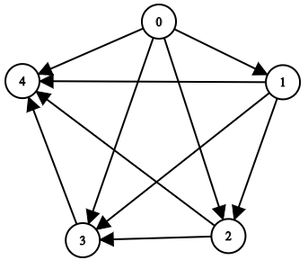
Input: n = 5, edgeList = [[0,1],[0,2],[0,3],[0,4],[1,2],[1,3],[1,4],[2,3],[2,4],[3,4]]
Output: [[],[0],[0,1],[0,1,2],[0,1,2,3]]
Explanation:
The above diagram represents the input graph.
- Node 0 does not have any ancestor.
- Node 1 has one ancestor 0.
- Node 2 has two ancestors 0 and 1.
- Node 3 has three ancestors 0, 1, and 2.
- Node 4 has four ancestors 0, 1, 2, and 3.
Constraints:
1 <= n <= 10000 <= edges.length <= min(2000, n * (n - 1) / 2)edges[i].length == 20 <= fromi, toi <= n - 1fromi != toi- There are no duplicate edges.
- The graph is directed and acyclic.
On This Page
Also Explore
DSA Questions
Number of Ways to Build Sturdy Brick Wall
DSA Questions
Counting Words With a Given Prefix
DSA Questions
Minimum Time to Complete Trips
DSA Questions
Minimum Time to Finish the Race
DSA Questions
Number of Ways to Build House of Cards
DSA Questions
Most Frequent Number Following Key In an Array
DSA Questions
Sort the Jumbled Numbers
DSA Questions
All Ancestors of a Node in a Directed Acyclic Graph
DSA Questions
Minimum Number of Moves to Make Palindrome
DSA Questions
Cells in a Range on an Excel Sheet
DSA Questions
Append K Integers With Minimal Sum
DSA Questions
Create Binary Tree From Descriptions
DSA Questions
Replace Non-Coprime Numbers in Array
DSA Questions
Number of Single Divisor Triplets
DSA Questions
Finding the Topic of Each Post
DSA Questions