{x}
blog image

Unique Paths III

You are given an m x n integer array grid where grid[i][j] could be:

  • 1 representing the starting square. There is exactly one starting square.
  • 2 representing the ending square. There is exactly one ending square.
  • 0 representing empty squares we can walk over.
  • -1 representing obstacles that we cannot walk over.

Return the number of 4-directional walks from the starting square to the ending square, that walk over every non-obstacle square exactly once.


Example 1:

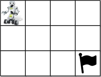
Input: grid = [[1,0,0,0],[0,0,0,0],[0,0,2,-1]]
Output: 2
Explanation: We have the following two paths: 
1. (0,0),(0,1),(0,2),(0,3),(1,3),(1,2),(1,1),(1,0),(2,0),(2,1),(2,2)
2. (0,0),(1,0),(2,0),(2,1),(1,1),(0,1),(0,2),(0,3),(1,3),(1,2),(2,2)

Example 2:

Input: grid = [[1,0,0,0],[0,0,0,0],[0,0,0,2]]
Output: 4
Explanation: We have the following four paths: 
1. (0,0),(0,1),(0,2),(0,3),(1,3),(1,2),(1,1),(1,0),(2,0),(2,1),(2,2),(2,3)
2. (0,0),(0,1),(1,1),(1,0),(2,0),(2,1),(2,2),(1,2),(0,2),(0,3),(1,3),(2,3)
3. (0,0),(1,0),(2,0),(2,1),(2,2),(1,2),(1,1),(0,1),(0,2),(0,3),(1,3),(2,3)
4. (0,0),(1,0),(2,0),(2,1),(1,1),(0,1),(0,2),(0,3),(1,3),(1,2),(2,2),(2,3)

Example 3:

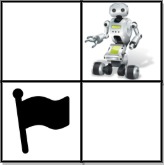
Input: grid = [[0,1],[2,0]]
Output: 0
Explanation: There is no path that walks over every empty square exactly once.
Note that the starting and ending square can be anywhere in the grid.


Constraints:

  • m == grid.length
  • n == grid[i].length
  • 1 <= m, n <= 20
  • 1 <= m * n <= 20
  • -1 <= grid[i][j] <= 2
  • There is exactly one starting cell and one ending cell.

980. Unique Paths III

Problem Description

Given an m x n integer array grid representing a grid where:

  • 1 represents the starting square.
  • 2 represents the ending square.
  • 0 represents empty squares.
  • -1 represents obstacles.

Find the number of 4-directional walks from the starting square to the ending square that walk over every non-obstacle square exactly once.

Solution: Backtracking

This problem can be efficiently solved using a backtracking algorithm. The core idea is to explore all possible paths from the starting point to the ending point, keeping track of visited cells. We only consider valid paths that visit every non-obstacle cell exactly once.

Algorithm

  1. Initialization:

    • Find the starting coordinates (start_row, start_col) and the ending coordinates.
    • Count the number of empty cells (empty_count). This helps us determine if a path is complete.
  2. Backtracking Function (dfs):

    • dfs(row, col, visited_count): This recursive function takes the current row and column, and the number of visited cells as input.
    • Base Cases:
      • If we reach the ending square (grid[row][col] == 2):
        • If visited_count equals empty_count + 1 (all empty cells and the start cell have been visited), we found a valid path, so return 1.
        • Otherwise, return 0 (incomplete path).
    • Recursive Step:
      • Iterate over the four neighboring cells (up, down, left, right).
      • For each neighbor:
        • Check if it's within bounds, not an obstacle (grid[neighbor_row][neighbor_col] != -1), and not already visited.
        • Mark the neighbor as visited.
        • Recursively call dfs on the neighbor.
        • Unmark the neighbor (backtracking step). This allows exploration of other paths.
    • Return the sum of valid paths found from all neighbors.
  3. Main Function:

    • Call the dfs function starting from the start_row, start_col, and an initial visited_count of 0.

Time and Space Complexity

  • Time Complexity: O(4N), where N is the number of empty cells. In the worst case, we explore all possible paths. The actual runtime is significantly smaller than this theoretical bound for most inputs because of early pruning with the visited_count check.
  • Space Complexity: O(N) due to the recursive call stack and the visited set (or similar data structure to track visited cells).

Code (Python)

def uniquePathsIII(grid):
    rows, cols = len(grid), len(grid[0])
    start_row, start_col = -1, -1
    empty_count = 0
 
    for r in range(rows):
        for c in range(cols):
            if grid[r][c] == 1:
                start_row, start_col = r, c
            elif grid[r][c] == 0:
                empty_count += 1
 
    def dfs(row, col, visited_count):
        if grid[row][col] == 2:
            return 1 if visited_count == empty_count + 1 else 0
 
        count = 0
        for dr, dc in [(0, 1), (0, -1), (1, 0), (-1, 0)]:
            new_row, new_col = row + dr, col + dc
            if 0 <= new_row < rows and 0 <= new_col < cols and grid[new_row][new_col] != -1:
                temp = grid[new_row][new_col]
                grid[new_row][new_col] = -1  # Mark as visited (temporarily)
 
                count += dfs(new_row, new_col, visited_count + 1)
 
                grid[new_row][new_col] = temp  # Backtrack
 
        return count
 
    return dfs(start_row, start_col, 0)
 

The code in other languages (Java, C++, Go, TypeScript, JavaScript) follows a very similar structure, using the same backtracking approach. The primary difference lies in syntax and data structure choices. The core logic remains consistent.