{x}
blog image

Shortest Path in Binary Matrix

Given an n x n binary matrix grid, return the length of the shortest clear path in the matrix. If there is no clear path, return -1.

A clear path in a binary matrix is a path from the top-left cell (i.e., (0, 0)) to the bottom-right cell (i.e., (n - 1, n - 1)) such that:

  • All the visited cells of the path are 0.
  • All the adjacent cells of the path are 8-directionally connected (i.e., they are different and they share an edge or a corner).

The length of a clear path is the number of visited cells of this path.


Example 1:

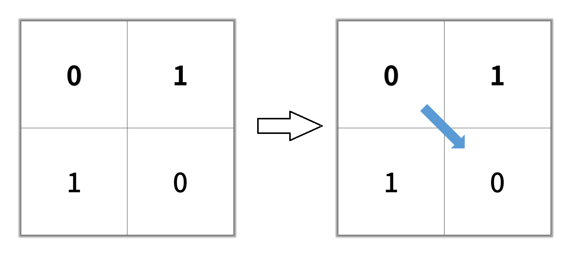
Input: grid = [[0,1],[1,0]]
Output: 2

Example 2:

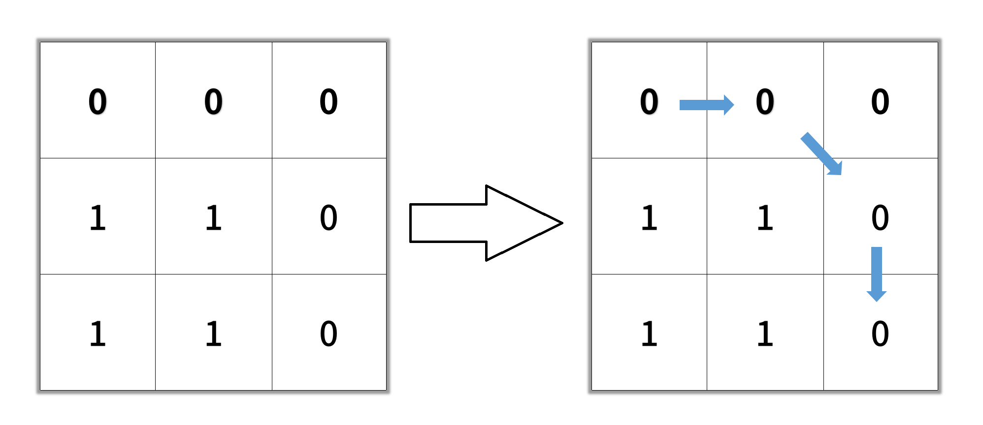
Input: grid = [[0,0,0],[1,1,0],[1,1,0]]
Output: 4

Example 3:

Input: grid = [[1,0,0],[1,1,0],[1,1,0]]
Output: -1


Constraints:

  • n == grid.length
  • n == grid[i].length
  • 1 <= n <= 100
  • grid[i][j] is 0 or 1

Solution Explanation: Shortest Path in Binary Matrix

This problem asks for the shortest path from the top-left to the bottom-right corner of a binary matrix, where only cells with value 0 can be traversed, and movement is allowed in all 8 directions.

The most efficient approach is using Breadth-First Search (BFS). BFS guarantees finding the shortest path in an unweighted graph (which our matrix represents).

Algorithm:

  1. Initialization:

    • Check if the starting cell grid[0][0] is 1 (blocked). If so, return -1 (no path).
    • Create a queue q and add the starting cell coordinates (0, 0) to it.
    • Mark grid[0][0] as visited (e.g., by setting its value to 1).
    • Initialize ans (path length) to 1.
  2. BFS Iteration:

    • While the queue q is not empty:
      • Process all cells added to the queue in the current level. This is done by iterating len(q) times in the loop.
      • For each cell (i, j) dequeued:
        • If (i, j) is the bottom-right cell (i == n - 1 && j == n - 1), return ans (shortest path found).
        • Explore all 8 neighbors of (i, j):
          • Check if the neighbor is within the matrix bounds (0 <= x < n and 0 <= y < n).
          • Check if the neighbor is not blocked (grid[x][y] == 0).
          • If both conditions are true:
            • Mark the neighbor as visited (grid[x][y] = 1).
            • Add the neighbor's coordinates to the queue q.
      • Increment ans (path length increases by one for each level).
  3. No Path:

    • If the queue becomes empty without finding the bottom-right cell, return -1 (no path exists).

Time Complexity Analysis:

  • In the worst-case scenario, BFS visits every cell in the matrix.
  • The time complexity is O(N^2), where N is the size of the matrix (N x N). This is because each cell might be visited and enqueued/dequeued once.

Space Complexity Analysis:

  • The space complexity is dominated by the queue q. In the worst-case, the queue can hold all cells in the matrix.
  • Therefore, the space complexity is O(N^2) as well.

Code Examples (with explanations inline):

The code examples in Python, Java, C++, Go, TypeScript, and Rust provided in the original response all implement this BFS algorithm effectively. They differ slightly in syntax and data structure usage (e.g., deque vs. queue, array vs. list), but the core logic remains the same. The in-line comments in the code provide further explanations.

The key improvement in these solutions compared to a simple recursive DFS is that BFS systematically explores the matrix level by level, guaranteeing that the shortest path is found first. DFS, on the other hand, can get trapped in exploring longer paths before finding the optimal solution.