{x}
blog image

Search a 2D Matrix

You are given an m x n integer matrix matrix with the following two properties:

  • Each row is sorted in non-decreasing order.
  • The first integer of each row is greater than the last integer of the previous row.

Given an integer target, return true if target is in matrix or false otherwise.

You must write a solution in O(log(m * n)) time complexity.


Example 1:

Input: matrix = [[1,3,5,7],[10,11,16,20],[23,30,34,60]], target = 3
Output: true

Example 2:

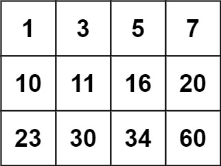
Input: matrix = [[1,3,5,7],[10,11,16,20],[23,30,34,60]], target = 13
Output: false


Constraints:

  • m == matrix.length
  • n == matrix[i].length
  • 1 <= m, n <= 100
  • -104 <= matrix[i][j], target <= 104

Solution Explanation for Search a 2D Matrix

The problem asks to determine if a target integer exists within a sorted 2D matrix. The matrix has the properties that each row is sorted in non-decreasing order, and the first integer of each row is greater than the last integer of the previous row. The solution must have a time complexity of O(log(m * n)), suggesting a binary search approach.

Approach 1: Binary Search on the Flattened Matrix

This approach treats the 2D matrix as a 1D sorted array. We perform a standard binary search on this "flattened" array to find the target.

Algorithm:

  1. Flatten conceptually: Imagine the matrix as a single sorted array.
  2. Binary Search: Apply binary search to this conceptual array. The mid index in the binary search needs to be converted back to row and column indices using integer division (// or /) and modulo (% or %).
  3. Comparison: Compare the element at the calculated (row, col) with the target. Adjust the search space (left or right) accordingly.
  4. Result: If the target is found, return true; otherwise, return false after the binary search completes.

Time Complexity: O(log(mn)) due to the binary search on the mn elements.

Space Complexity: O(1) because we use only a few variables for the search.

Approach 2: Linear Search from Bottom-Left or Top-Right

This approach cleverly uses the sorted nature of the matrix to perform a linear search with a directional strategy.

Algorithm:

  1. Start Point: Begin at either the bottom-left or top-right corner of the matrix. The choice doesn't affect the complexity but might subtly change the number of comparisons.
  2. Comparison and Movement: Compare the current element with the target:
    • If equal, return true.
    • If greater than the target, move upward (decrement row index) if starting from bottom-left or move left (decrement column index) if starting from top-right.
    • If less than the target, move right (increment column index) if starting from bottom-left or move down (increment row index) if starting from top-right.
  3. Termination: The search terminates when you reach the boundary of the matrix without finding the target. Return false.

Time Complexity: O(m+n) in the worst case. This is because you might traverse the entire last row or first column of the matrix, making this slightly less efficient than the binary search method when the matrix is large.

Space Complexity: O(1) as we use constant extra space.

Code Examples (Python)

Approach 1: Binary Search

def searchMatrix(matrix, target):
    m, n = len(matrix), len(matrix[0])
    left, right = 0, m * n - 1
    while left <= right:
        mid = (left + right) // 2
        row, col = divmod(mid, n)  #Convert 1D index to 2D indices
        if matrix[row][col] == target:
            return True
        elif matrix[row][col] < target:
            left = mid + 1
        else:
            right = mid - 1
    return False

Approach 2: Linear Search from Bottom-Left

def searchMatrix(matrix, target):
    rows, cols = len(matrix), len(matrix[0])
    row, col = rows - 1, 0  #Start from bottom-left
    while row >= 0 and col < cols:
        if matrix[row][col] == target:
            return True
        elif matrix[row][col] > target:
            row -= 1 #Move up
        else:
            col += 1 #Move right
    return False
 

Both approaches correctly solve the problem. Approach 1 (binary search) is generally preferred due to its guaranteed logarithmic time complexity, making it more efficient for larger matrices. Approach 2 might be slightly faster in practice for very small matrices, but its linear time complexity makes it less scalable. The choice depends on the anticipated size of the input matrix.