{x}
blog image

Reachable Nodes In Subdivided Graph

You are given an undirected graph (the "original graph") with n nodes labeled from 0 to n - 1. You decide to subdivide each edge in the graph into a chain of nodes, with the number of new nodes varying between each edge.

The graph is given as a 2D array of edges where edges[i] = [ui, vi, cnti] indicates that there is an edge between nodes ui and vi in the original graph, and cnti is the total number of new nodes that you will subdivide the edge into. Note that cnti == 0 means you will not subdivide the edge.

To subdivide the edge [ui, vi], replace it with (cnti + 1) new edges and cnti new nodes. The new nodes are x1, x2, ..., xcnti, and the new edges are [ui, x1], [x1, x2], [x2, x3], ..., [xcnti-1, xcnti], [xcnti, vi].

In this new graph, you want to know how many nodes are reachable from the node 0, where a node is reachable if the distance is maxMoves or less.

Given the original graph and maxMoves, return the number of nodes that are reachable from node 0 in the new graph.


Example 1:

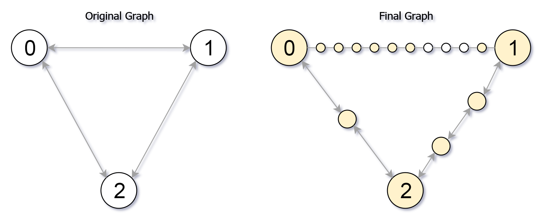
Input: edges = [[0,1,10],[0,2,1],[1,2,2]], maxMoves = 6, n = 3
Output: 13
Explanation: The edge subdivisions are shown in the image above.
The nodes that are reachable are highlighted in yellow.

Example 2:

Input: edges = [[0,1,4],[1,2,6],[0,2,8],[1,3,1]], maxMoves = 10, n = 4
Output: 23

Example 3:

Input: edges = [[1,2,4],[1,4,5],[1,3,1],[2,3,4],[3,4,5]], maxMoves = 17, n = 5
Output: 1
Explanation: Node 0 is disconnected from the rest of the graph, so only node 0 is reachable.


Constraints:

  • 0 <= edges.length <= min(n * (n - 1) / 2, 104)
  • edges[i].length == 3
  • 0 <= ui < vi < n
  • There are no multiple edges in the graph.
  • 0 <= cnti <= 104
  • 0 <= maxMoves <= 109
  • 1 <= n <= 3000

Solution Explanation for Reachable Nodes In Subdivided Graph

This problem involves finding the number of reachable nodes in a graph after subdividing its edges. The solution uses Dijkstra's algorithm with a priority queue (heap) to efficiently find the shortest distances from the starting node (0) to all other nodes in the modified graph.

Approach:

  1. Graph Representation: The input edges is represented as an adjacency list. Each edge [u, v, cnt] is added to the adjacency list for both u and v. The cnt value represents the number of nodes to insert between u and v when subdividing.

  2. Subdivision Simulation: The solution doesn't explicitly create the subdivided graph. Instead, it simulates the subdivision during the Dijkstra's algorithm execution. When exploring an edge (u, v, cnt), the algorithm considers the total distance to reach v as dist[u] + cnt + 1.

  3. Dijkstra's Algorithm: A priority queue is used to efficiently manage nodes to explore. The queue stores pairs (distance, node). The algorithm iteratively picks the node with the minimum distance and updates distances to its neighbors.

  4. Reachable Nodes Count: After Dijkstra's, the number of nodes reachable within maxMoves is counted.

  5. Edge Contribution: The algorithm accounts for nodes added during edge subdivisions that might be reachable even if their adjacent original nodes aren't. For each edge (u, v, cnt), it calculates how many newly added nodes along this edge are within reach, considering the distances from both ends (u and v).

Time Complexity Analysis:

  • Graph Construction: O(E), where E is the number of edges in the input.
  • Dijkstra's Algorithm: O(E log V), where V is the number of nodes (n). The log V factor comes from using a heap.
  • Edge Contribution Calculation: O(E).

Therefore, the overall time complexity is O(E log V), dominated by Dijkstra's algorithm.

Space Complexity Analysis:

  • Adjacency List: O(E)
  • Distance Array: O(V)
  • Priority Queue: O(V) in the worst case.

Therefore, the overall space complexity is O(E + V).

Code Explanation (Python):

import heapq
from collections import defaultdict
 
class Solution:
    def reachableNodes(self, edges: List[List[int]], maxMoves: int, n: int) -> int:
        g = defaultdict(list)  # Adjacency list
        for u, v, cnt in edges:
            g[u].append((v, cnt + 1)) # +1 to include the original edge weight
            g[v].append((u, cnt + 1))
 
        q = [(0, 0)] # (distance, node)
        dist = [float('inf')] * n  # Initialize distances to infinity
        dist[0] = 0  # Distance from 0 to 0 is 0
 
        while q:
            d, u = heapq.heappop(q) # Get node with smallest distance
            if d > maxMoves:
                break # Optimization: Stop if current distance exceeds maxMoves
 
            for v, cnt in g[u]:
                if d + cnt < dist[v]:
                    dist[v] = d + cnt
                    heapq.heappush(q, (dist[v], v))
 
        ans = sum(1 for d in dist if d <= maxMoves)  # Count reachable nodes
 
        for u, v, cnt in edges:
            a = min(cnt, max(0, maxMoves - dist[u])) # Nodes reachable from u
            b = min(cnt, max(0, maxMoves - dist[v])) # Nodes reachable from v
            ans += min(cnt, a + b) # Add nodes reachable from both ends
 
        return ans
 

The other language versions (Java, C++, Go) follow a similar structure, adapting the syntax and data structures to their respective languages. The core algorithm remains the same. Note the use of efficient data structures like priority queues (heap) to optimize the Dijkstra's algorithm, crucial for handling larger graphs efficiently.