
Number of Orders in the Backlog
You are given a 2D integer array orders, where each orders[i] = [pricei, amounti, orderTypei] denotes that amounti orders have been placed of type orderTypei at the price pricei. The orderTypei is:
0if it is a batch ofbuyorders, or1if it is a batch ofsellorders.
Note that orders[i] represents a batch of amounti independent orders with the same price and order type. All orders represented by orders[i] will be placed before all orders represented by orders[i+1] for all valid i.
There is a backlog that consists of orders that have not been executed. The backlog is initially empty. When an order is placed, the following happens:
- If the order is a
buyorder, you look at thesellorder with the smallest price in the backlog. If thatsellorder's price is smaller than or equal to the currentbuyorder's price, they will match and be executed, and thatsellorder will be removed from the backlog. Else, thebuyorder is added to the backlog. - Vice versa, if the order is a
sellorder, you look at thebuyorder with the largest price in the backlog. If thatbuyorder's price is larger than or equal to the currentsellorder's price, they will match and be executed, and thatbuyorder will be removed from the backlog. Else, thesellorder is added to the backlog.
Return the total amount of orders in the backlog after placing all the orders from the input. Since this number can be large, return it modulo 109 + 7.
Example 1:
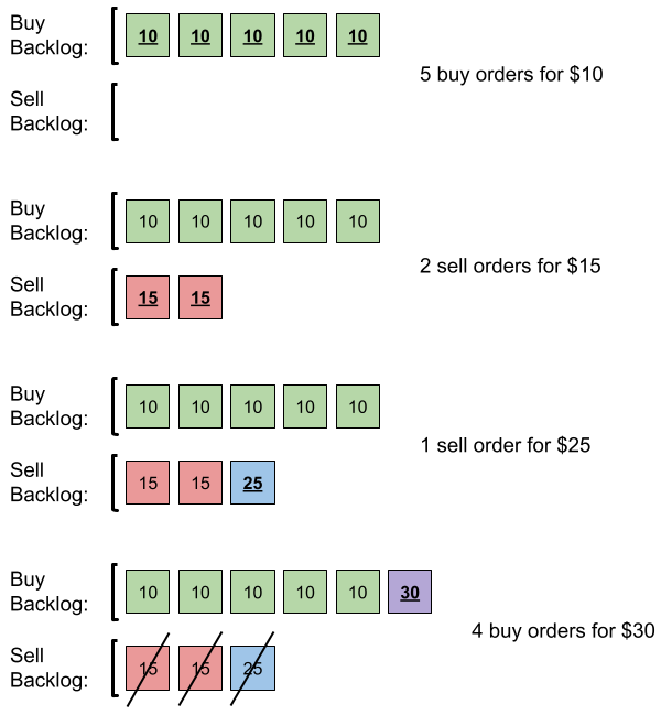
Input: orders = [[10,5,0],[15,2,1],[25,1,1],[30,4,0]]
Output: 6
Explanation: Here is what happens with the orders:
- 5 orders of type buy with price 10 are placed. There are no sell orders, so the 5 orders are added to the backlog.
- 2 orders of type sell with price 15 are placed. There are no buy orders with prices larger than or equal to 15, so the 2 orders are added to the backlog.
- 1 order of type sell with price 25 is placed. There are no buy orders with prices larger than or equal to 25 in the backlog, so this order is added to the backlog.
- 4 orders of type buy with price 30 are placed. The first 2 orders are matched with the 2 sell orders of the least price, which is 15 and these 2 sell orders are removed from the backlog. The 3rd order is matched with the sell order of the least price, which is 25 and this sell order is removed from the backlog. Then, there are no more sell orders in the backlog, so the 4th order is added to the backlog.
Finally, the backlog has 5 buy orders with price 10, and 1 buy order with price 30. So the total number of orders in the backlog is 6.
Example 2:
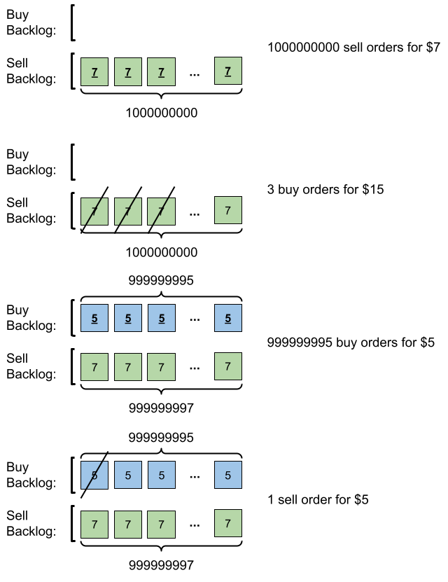
Input: orders = [[7,1000000000,1],[15,3,0],[5,999999995,0],[5,1,1]]
Output: 999999984
Explanation: Here is what happens with the orders:
- 109 orders of type sell with price 7 are placed. There are no buy orders, so the 109 orders are added to the backlog.
- 3 orders of type buy with price 15 are placed. They are matched with the 3 sell orders with the least price which is 7, and those 3 sell orders are removed from the backlog.
- 999999995 orders of type buy with price 5 are placed. The least price of a sell order is 7, so the 999999995 orders are added to the backlog.
- 1 order of type sell with price 5 is placed. It is matched with the buy order of the highest price, which is 5, and that buy order is removed from the backlog.
Finally, the backlog has (1000000000-3) sell orders with price 7, and (999999995-1) buy orders with price 5. So the total number of orders = 1999999991, which is equal to 999999984 % (109 + 7).
Constraints:
1 <= orders.length <= 105orders[i].length == 31 <= pricei, amounti <= 109orderTypeiis either0or1.