There is a bi-directional graph with n
vertices, where each vertex is labeled from 0
to n - 1
(inclusive). The edges in the graph are represented as a 2D integer array edges
, where each edges[i] = [ui, vi]
denotes a bi-directional edge between vertex ui
and vertex vi
. Every vertex pair is connected by at most one edge, and no vertex has an edge to itself.
You want to determine if there is a valid path that exists from vertex source
to vertex destination
.
Given edges
and the integers n
, source
, and destination
, return true
if there is a valid path from source
to destination
, or false
otherwise.
Example 1:
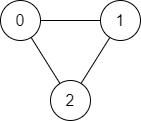
Input: n = 3, edges = [[0,1],[1,2],[2,0]], source = 0, destination = 2 Output: true Explanation: There are two paths from vertex 0 to vertex 2: - 0 → 1 → 2 - 0 → 2
Example 2:
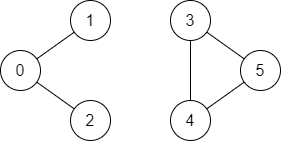
Input: n = 6, edges = [[0,1],[0,2],[3,5],[5,4],[4,3]], source = 0, destination = 5 Output: false Explanation: There is no path from vertex 0 to vertex 5.
Constraints:
1 <= n <= 2 * 105
0 <= edges.length <= 2 * 105
edges[i].length == 2
0 <= ui, vi <= n - 1
ui != vi
0 <= source, destination <= n - 1
Given a graph represented as an adjacency list, determine if a path exists between a source and destination node.
Three approaches are presented: Depth-First Search (DFS), Breadth-First Search (BFS), and Union-Find.
This recursive approach explores the graph depth-wise.
Algorithm:
edges
into an adjacency list g
where g[i]
contains all neighbors of node i
.i
is the destination
, return true
.i
as visited in the vis
set.dfs
for each unvisited neighbor of i
. If any recursive call returns true
, return true
.destination
is found from the current node, return false
.dfs(source)
to start the search.Time Complexity: O(V + E), where V is the number of vertices (nodes) and E is the number of edges. This is because each node and edge is visited at most once.
Space Complexity: O(V + E) in the worst case due to the recursion stack and the adjacency list. In practice, the space usage is often less than this due to tail-call optimization in some languages.
Code (Python):
class Solution:
def validPath(self, n: int, edges: List[List[int]], source: int, destination: int) -> bool:
g = [[] for _ in range(n)]
for u, v in edges:
g[u].append(v)
g[v].append(u)
vis = set()
def dfs(i: int) -> bool:
if i == destination:
return True
vis.add(i)
for j in g[i]:
if j not in vis and dfs(j):
return True
return False
return dfs(source)
Code (Java):
class Solution {
private int destination;
private boolean[] vis;
private List<Integer>[] g;
public boolean validPath(int n, int[][] edges, int source, int destination) {
this.destination = destination;
vis = new boolean[n];
g = new ArrayList[n];
Arrays.setAll(g, i -> new ArrayList<>());
for (int[] e : edges) {
int u = e[0], v = e[1];
g[u].add(v);
g[v].add(u);
}
return dfs(source);
}
private boolean dfs(int i) {
if (i == destination) {
return true;
}
vis[i] = true;
for (int j : g[i]) {
if (!vis[j] && dfs(j)) {
return true;
}
}
return false;
}
}
Similar code can be written in other languages following the same logic.
This iterative approach explores the graph level by level.
Algorithm:
q
with the source
node.vis
set to track visited nodes. Add source
to vis
.i
.i
is the destination
, return true
.j
of i
:
j
to q
and vis
.destination
, return false
.Time Complexity: O(V + E). Similar to DFS, each node and edge is visited at most once.
Space Complexity: O(V) in the worst case because the queue can contain at most all nodes. The vis
set also uses O(V) space.
Code (Python):
from collections import deque
class Solution:
def validPath(self, n: int, edges: List[List[int]], source: int, destination: int) -> bool:
g = [[] for _ in range(n)]
for u, v in edges:
g[u].append(v)
g[v].append(u)
q = deque([source])
vis = {source}
while q:
i = q.popleft()
if i == destination:
return True
for j in g[i]:
if j not in vis:
vis.add(j)
q.append(j)
return False
This approach uses a disjoint-set data structure to efficiently determine connectivity.
Algorithm:
UnionFind
data structure with n
nodes.edges
. For each edge (u, v)
, merge the sets containing u
and v
using the union
operation of the UnionFind
structure.source
and destination
belong to the same set using the find
operation. If they do, there is a path; otherwise, there isn't.Time Complexity: The time complexity is dominated by the union
and find
operations. A well-implemented Union-Find structure achieves amortized time complexity of almost O(1) for each operation using path compression and union by rank. Therefore, the overall time complexity is O(E + V), where E is the number of edges, and V is the number of vertices.
Space Complexity: O(V) to store the parent array in the Union-Find data structure.
Code (Python):
class UnionFind:
def __init__(self, n):
self.parent = list(range(n))
self.rank = [0] * n
def find(self, i):
if self.parent[i] == i:
return i
self.parent[i] = self.find(self.parent[i])
return self.parent[i]
def union(self, i, j):
root_i = self.find(i)
root_j = self.find(j)
if root_i != root_j:
if self.rank[root_i] < self.rank[root_j]:
self.parent[root_i] = root_j
elif self.rank[root_i] > self.rank[root_j]:
self.parent[root_j] = root_i
else:
self.parent[root_j] = root_i
self.rank[root_i] += 1
return True
return False
class Solution:
def validPath(self, n: int, edges: List[List[int]], source: int, destination: int) -> bool:
uf = UnionFind(n)
for u, v in edges:
uf.union(u, v)
return uf.find(source) == uf.find(destination)
Remember to adapt the Union-Find implementation details for other languages, as the specifics might differ slightly. However, the core algorithm remains the same. The provided Python code shows a path compression and union by rank optimized version for better performance.