
Add One Row to Tree
Given the root of a binary tree and two integers val and depth, add a row of nodes with value val at the given depth depth.
Note that the root node is at depth 1.
The adding rule is:
- Given the integer
depth, for each not null tree nodecurat the depthdepth - 1, create two tree nodes with valuevalascur's left subtree root and right subtree root. cur's original left subtree should be the left subtree of the new left subtree root.cur's original right subtree should be the right subtree of the new right subtree root.- If
depth == 1that means there is no depthdepth - 1at all, then create a tree node with valuevalas the new root of the whole original tree, and the original tree is the new root's left subtree.
Example 1:
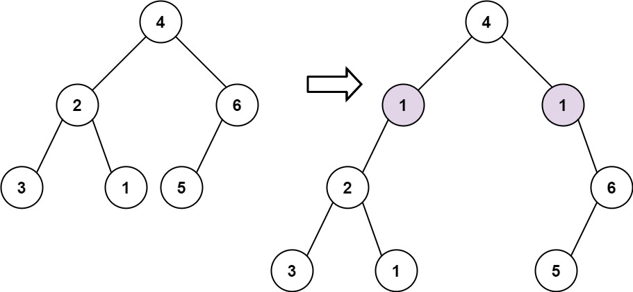
Input: root = [4,2,6,3,1,5], val = 1, depth = 2
Output: [4,1,1,2,null,null,6,3,1,5]
Example 2:
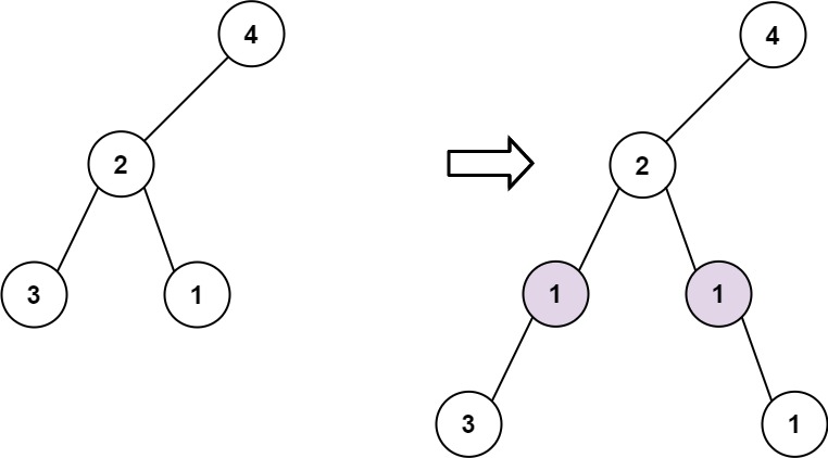
Input: root = [4,2,null,3,1], val = 1, depth = 3
Output: [4,2,null,1,1,3,null,null,1]
Constraints:
- The number of nodes in the tree is in the range
[1, 104]. - The depth of the tree is in the range
[1, 104]. -100 <= Node.val <= 100-105 <= val <= 1051 <= depth <= the depth of tree + 1
On This Page
Also Explore
DSA Questions
Average Salary: Departments VS Company
DSA Questions
Add Bold Tag in String
DSA Questions
Merge Two Binary Trees
DSA Questions
Students Report By Geography
DSA Questions
Biggest Single Number
DSA Questions
Not Boring Movies
DSA Questions
Task Scheduler
DSA Questions
Design Circular Queue
DSA Questions
Add One Row to Tree
DSA Questions
Maximum Distance in Arrays
DSA Questions
Minimum Factorization
DSA Questions
Exchange Seats
DSA Questions
Swap Salary
DSA Questions
Maximum Product of Three Numbers
DSA Questions
K Inverse Pairs Array
DSA Questions
Course Schedule III
DSA Questions